Taking the confusion out of determining appropriate data collection parameters.
In 1924, Dr. Walter Shewhart was working at Bell Telephone Laboratories. On May 16 of that year, Dr. Shewhart wrote a memorandum in which he presented and proposed the process control chart to his superiors. Bell Telephone Laboratories believed this memorandum gave it a competitive advantage and held this paper internally. In 1931, Dr. Shewhart published his book Economic Control of Quality of Manufactured Product. In this book, Dr. Shewhart explained in detail the fundamental concepts and benefits of statistical process control. This seminal work laid the foundation for the modern quality control discipline, and the process control chart became the bedrock of quality control systems.
The most critical assumption made concerning statistical process control (SPC) charts, i.e., Shewhart Control Charts, is that of data independence from one observation to the next (not autocorrelated).1,2 The second assumption is that the individual observations are approximately normally distributed.1,2 The tabled constants used to calculate the SPC chart limits are constructed under the assumption of independence and normality.
Conventional SPC charts do not work well if the quality attributes charted exhibit even low levels of correlation over time. Correlated data produce too many false alarms. Of important note on the Shewhart +/-3-sigma SPC chart is that 99.73% of the data are contained within this interval. The 99.73%, or 0.9973, is the probability of not receiving a signal when the process is in control, the data are not autocorrelated, and normality is assumed.
Many printed circuit board chemical manufacturing processes can violate the assumption of uncorrelated observations (autocorrelation). This is because inertial elements drive reduction-oxidation (redox) chemical processes. When the interval between samples becomes small relative to the inertial elements, the sequential observations of the process will be correlated over time. Autocorrelation can result from assignable causes, too; e.g., malfunctioning equipment, wrong adds.
Sampling Frequency
Sampling frequency depends upon the cost of sampling, the losses associated with allowing the process to operate out of control, the rate of production, and the potential for process shifts to occur. There are no hard rules that one needs to sample n consecutive samples every x number of cycles. The general belief is that if the interval between samples is too great, defective products could be produced before another opportunity to detect the process shift occurs.
The most feasible way to detect mean shifts is to take large samples frequently, which is usually not economically viable. Generally, we take small samples at short intervals or larger samples at longer intervals. Current industry practice favors smaller, more frequent samples, particularly in high-volume manufacturing processes or where multiple assignable causes can occur.
According to the US DoD Handbook Companion Document to Mil-Std-1916, the following factors should be considered when determining sampling frequency3:
Process change rapidity. The smaller the interval between inherent process changes, the smaller the interval between subgroups.
Relative variability of the process. If the process variability is minimal and the chance of producing an out-of-specification product is negligible, then such a process may be monitored infrequently. This is beneficial when the cost of sampling and testing is high.
Initial data collection. At first, it may be desirable to sample frequently to arrive at conclusions quickly. After sufficient process knowledge is gained, reducing the frequency of sampling may be advisable.
Potential nonconforming product. How much product a supplier can produce between the beginning of a change in process average and the detection of that change should influence the sampling interval. This relates to factors such as production rates and inspection and rework costs.
Sampling Subgroup
Rational subgroups should be selected so that if assignable causes are present, the chance for differences between subgroups will be maximized, while differences due to assignable causes within a subgroup will be minimized.1 The preferred method for subgrouping consists of parts produced at the same time (or as close together as possible), ideally taking consecutive production units. Data from different operators, shifts and machines should not be mixed.2 Taking repeated measurements on a single part is not a rational subgroup.
Choosing the subgroup size is primarily based on allocating sampling effort. The available resources must be considered when determining subgroup size. Therefore, the subgroup size is generally not determined analytically but rather by convenience.2 In general, larger subgroup sizes will make detecting smaller shifts in the process easier. Many processes do not require great sensitivity in the detection of small shifts as these may occur from day to day. Hence, using larger subgroups may be counterproductive when too much time is spent checking the process for insignificant changes signaled by an oversensitive chart. Subgroups between 3 and 5 for x-bar charts and a subgroup of 1 for individual moving range charts are standard.
Subgroup sizes can be calculated using EQUATION 1.2 Detecting shifts in control charts is known as Power – the probability of detecting an out-of-control condition when the process is unstable. Power is calculated as 1– β (beta).

where:
n = subgroup size
Zα/2 = Type I error probability (out-of-control signal, but the process is stable)
Zβ = Type II error probability (failure to detect an out-of-control condition when the process is unstable)
σ = standard deviation of the characteristic being charted
D = difference to detect
Ζ values can be found in a standard normal table in any statistics textbook. There are no hard-and-fast rules about how much power is enough, but there does seem to be a consensus. Power should be greater than 50%, power of 80% is judged to be adequate, and power greater than 90% may waste resources.
Using an alpha (α) value of 0.0027 (corresponding to a standard Shewhart +/-3-sigma control chart) and holding the beta (β) values at 0.50 (power = 1 – 0.5 = 50%) and 0.20 (power = 1 – 0.2 = 80%), the charts in FIGURES 1 and 2 were produced for comparison purposes.
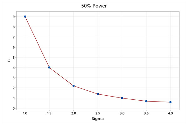
Figure 1. Subgroup size (n) with 50% power to detect a given sigma shift (x).

Figure 2. Subgroup size (n) with 80% power to detect a given sigma shift (x).
For example, using a subgroup of n = 1, a SPC chart has 50% power to detect a 3-sigma mean process shift on the first sample following the shift. The same chart has 80% power to detect a 4-sigma mean process shift on the first sample following the shift. The probability of detecting the shift increases with each consecutive sample.
Sampling Plan
A general starting point for discussing sampling plans is to use a sampling rate per unit of time of n/d = 1.0, where n = the number of samples in the subgroup and d = the sampling interval. The choices of n and d affect the costs associated with the sampling plan and the ability of the control chart to detect process changes. A critical decision in designing the sampling plan is choosing between taking subgroup sizes of n = 1 or n >1.
When detecting a sustained shift is of interest, the best performance is obtained using subgroups of moderate sizes, such as n = 4 and d = 4, with rational subgrouping employed. When detecting transient shifts of short duration is of interest (t < 4, where t = time units), the best performance is obtained using a subgroup of small sizes, such as n = 1 and d = 1. For PCB wet chemical process manufacturing, a general starting point for discussing the sampling plan is to use a sampling rate per unit of time of n/d = 0.25, where n = 1, and d = 4hr, or n/d = 0.50, where n = 3, and d = 6hr. Once the sampling plan has been established, one can move to Phase 1 and, ultimately, Phase 2 of statistical process control.
Phase 1, retrospective analysis, is designed to bring a process into a state of statistical control. This is accomplished by collecting 20 to 25 subgroups of size n, computing the control limits, and plotting the data. Note: Fewer than 20 subgroups produce control limits that are not as reliable.
These control limits are considered trial control limits and allow determination of whether the process was in control when the initial samples were selected. Points that are outside the control limits are investigated for assignable causes. Points with assignable causes that can be corrected by engineering and operators are removed. Control limits are then recalculated, and new data are collected and charted. Sometimes this will take several cycles in which the control chart is created, assignable causes are detected and corrected, revised control limits are calculated, and new data are collected and charted. Suppose all original data points plot inside the control limits and no systematic behavior is evident. In that case, one can conclude that the process was in control and the trial control limits are suitable for controlling future production. Once a clean set of data that represents in-control process performance has been demonstrated, one can move to Phase 2.
Phase 2, process monitoring, has an established set of reliable control limits. The control chart can be used for monitoring future production. Effectively using control charts requires periodic review and potential revision of the control limits and center line. One should establish regular periods for this review and possible modification of control chart limits, such as every month, every six months, or every 50 or 100 samples. When revising control limits, remember that using at least 25 subgroups for computing control limits is highly recommended.
Conclusions
Statistical process control charts have been in use for nearly 100 years. These charts are powerful tools, but it can be confusing to determine the appropriate data collection parameters.
Understanding the tradeoffs of the sampling frequency, subgroups, and plans is critical for controlling PCB manufacturing processes. As a starting point for discussing the sampling plan, using a sampling rate per unit of time of n/d = 0.25, where n = 1, d = 4 hours, or n/d = 0.50, where n = 3, and d = 6 hours is recommended. Systematically moving from Phase 1 to Phase 2 ensures establishing proper control limits and maintaining them. Regular periods for review and revision of control chart limits enhance continuous improvement efforts.
References
1. D. Montgomery, Introduction to Statistical Quality Control, 6th Ed., John Wiley & Sons, 2009.
2. T. Ryan, Statistical Methods for Quality Improvement, 2nd Ed., John Wiley & Sons, 2000.
3. US Department of Defense, Handbook Companion Document to Mil-Std-1916 (DoD Publication No. MIL-HDBK-1916), 1999.
PATRICK VALENTINE, PH.D., is technical and Lean Six Sigma manager at Uyemura USA (uyemura.com); This email address is being protected from spambots. You need JavaScript enabled to view it.. He holds a doctorate in Quality Systems Management from New England College of Business and ASQ certifications as a Six Sigma Black Belt and Reliability Engineer.