Many of the values we want to estimate are unknowable because the parameters themselves are unknown.

I am often asked, “What is the accuracy of your (abc) calculator?” On the surface, this is a simple question. The answer is +/-xx%. If we dig a little deeper, it is kind of a loaded question; accuracy compared to what? If we dig even deeper, it gets even more complicated. What do we really mean? For an impedance calculator, for example, we want to know how accurate the estimate is to the actual (true) impedance, or we want to know how wide to make the trace to hit a specific (true) impedance. For a trace temperature calculator, we want to know how accurate the temperature estimate is compared to the actual (true) temperature.

There are two really significant problem areas here when we ask this question. The first is most people don’t fully grasp the difference between the layman’s use of the term accuracy compared to the relationship between the proper use of accuracy and its closely related cousin precision. The second is stating the accuracy of our estimate implies the actual measurement (of impedance or temperature, for example); i.e., the truth is known or knowable. In practical fact, we often have calculators that have excellent (say 1%) precision trying to estimate parameters that are only knowable within about 10%!

Here we discuss the complexities of each of these areas.

Accuracy vs. Precision

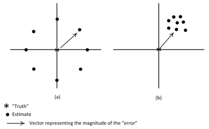
If you look up “accuracy,” the definitions given are usually related to the “closeness” of the estimate to the actual.¹ In many references, precision is listed as a synonym for accuracy. But technically there is a significant difference between these terms. It is easiest to show the difference in a diagram (FIGURE 1).

Figure 1. Difference between accuracy and precision.

In Figure 1, each side illustrates a position of “truth” with various estimates around it. In Figure 1a, the estimates are all equidistant away from the “truth,” the degree of error represented by the length of the vector. If we add up all the estimates and divide by n (resulting in the mean estimate²), we get the same value as “truth.” Figure 1a shows a high degree of accuracy; the mean estimate is the same as truth, even though no estimate is particularly close to the truth.

In Figure 1b, we have estimates that are closely grouped together, although they are all some distance away from the truth. If we calculate the mean estimate, it is somewhere in the upper right quadrant, some distance from the truth. Figure 1b illustrates a high degree of precision; all the estimates are clustered closely together. But Figure 1b shows a significant bias away from truth.

So, Figure 1a illustrates estimates with high accuracy but poor precision, while Figure 1b illustrates estimates with high precision but poor accuracy. Obviously, what we want is an estimating procedure that has both high accuracy and high precision. When we simply ask “how accurate is your estimate?” we are implicitly assuming the estimate is unbiased, and we are actually asking about the precision.

What is ‘Truth?’

Stating an expected range of “accuracy” implies we know, or can know, the true value. It assumes that at some prior time, we compared estimated values to the true values. So one question is: Is this actually possible?

Intuitively it certainly seems so. With an impedance calculator, for example, we build a test board with test traces, measure the impedance of the traces, and compare the result with a value derived from some estimating procedure (e.g., calculator). The most important parameters determining trace impedance are trace width, distance from one or more planes, and relative dielectric coefficient of the material around the trace. (Trace thickness has a secondary impact.) So knowing “truth” involves also knowing these parameters. We assume we know them based on the design specifications of the test board/trace. But in fact, there might well be variations that we are unaware of around the design parameters.

With a trace temperature calculator, it is the same thing. We build a test board or several test traces, measure the trace temperature for a given current, and then compare the measured values with the calculated ones. But measuring/estimating trace temperatures can be even more complicated. First, how do we measure trace temperature? There are three typical, reasonably practical ways we can do so: a) the “change of resistance” method (following IPC-TM-650³), b) using a thermocouple probe, or c) using an infrared measuring tool. Each has its limitations. The most obvious difference among them is that procedure (a) measures the “average” temperature along the length of the (test section of the) trace. If there is a thermal gradient along the trace, (a) averages the gradient. On the other hand, (b) and (c) measure the temperature at a point along the trace, which may or may not be the hottest point along the trace. Each has its own degree of inherent “accuracy.”

The most important parameters affecting trace temperature are copper thickness, trace width, copper resistivity, the thermal conductivity coefficient (in two axes, Tcon_x,y and Tcon_z) of the dielectric material under the trace, and the heat transfer coefficient (HTC) of the heat into the air (or vacuum) above the trace.⁴ From personal experience, the only parameters that are even somewhat straightforward are trace width and (possibly) copper resistivity. There are real problems knowing any of the others.

Therefore, how confident can we be that we know the “truth” around which we are comparing our estimates? But all this is the easy part! The more difficult part is that both trace impedance and trace temperature are “point” concepts. That is, both impedance and temperature can be different at each point along a trace. The impedance change of the trace shown in FIGURE 2 is obvious: The impedance of the trace changes at the point where the width of the trace changes.

Figure 2. Portion of a trace on a PCB. The impedance of this trace changes at the point where the width of the trace changes.

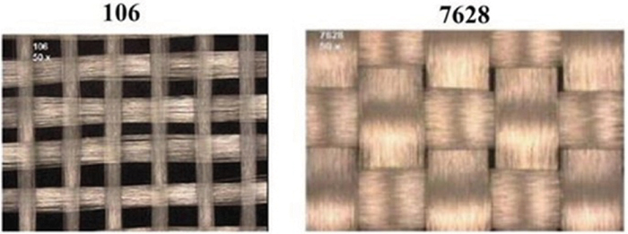
Less obvious is the impedance of a trace can change anywhere along the trace where the fiber weave of the dielectric changes (FIGURE 3). The variations of impedance and propagation speed as a function of fiberglass weave are well understood. A Web search for fiber weave effect on PCBs will result in thousands of hits. The e_r for the fiberglass is roughly 6, while the er for the resin in the dielectric is more like 3.5. On average, the resultant er is about 4.2, which is the rule of thumb we all use for FR-4. As a trace crosses over the “open” and “closed” areas of the weave, the impedance and propagation speed along the trace can vary. This becomes more important as the rise time of the signal decreases. Therefore, the concept of “true” impedance becomes more obscure.

Figure 3. Fiber weave that makes up a PCB dielectric for glass styles 106 and 7628, respectively.⁵

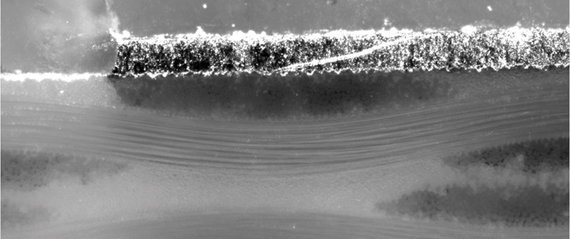
In addition, the roughness of the underlying surface of the copper trace (FIGURE 4) can also impact the point impedance for signals with very fast rise times. I don’t want to overstate this particular issue. With good design practices, good fabrication control and thorough knowledge of the materials being used, we can still have pretty accurate knowledge of the impedance along a trace. But there are limits because there are variables that are very difficult to know and/or control.

Figure 4. Roughness between a 2.0 oz. foil trace and the board laminate. (Source: Brooks and Adam)

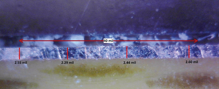
But the situation is much more difficult for knowing the “true” temperature. As stated above, several variables that affect temperature are difficult to know. Tconx,y and Tconz are rarely specified on datasheets. There is still a lot to learn about HTC as it relates to traces on a PCB. Copper resistivity can vary by as much as 10% across a PCB, and thickness can vary by as much as 50%.⁴ FIGURE 5 illustrates a 40-mil long section of a 2.0 oz., 100-mil wide trace on a test PCB. The thickness varies from 2.29 to 2.60 mils just over this short section, an almost 12% variation. This case is typical of what can be seen on most PCBs, especially on the top layer with plated copper over copper foil.

Figure 5. Microsection of a portion of a 2.0 oz, 100-mil wide trace on a PCB. The variation in thickness ranges by almost 12% over this short section.

Variations in trace temperature along a trace are most dependent on trace thickness. The variations shown in Figure 5 can result in temperature non-uniformities like those shown in FIGURE 6. The trace temperature not only varies along the trace, but it does so even between the midpoint to the edge of the trace. And the (true) thickness of the trace is virtually unknowable. With present technologies, we can only “know” the thickness of a trace by microsectioning the trace – a destructive process. And if we do so, there is no reason to believe the same point on the same trace on another board in the same production lot will be exactly the same thickness.

Figure 6. Thermal image of a 100-mil wide, 0.5 oz trace raised from 25°C to roughly 49°C. (Source: Brooks and Adam)

So when we ask how accurately we can estimate the (true) temperature of a trace, we must be willing to accept the fact that the “true” temperature can only be known within some finite degree of error, which might be much greater than the accuracy of our estimating tool – e.g., calculator – itself. The uncomfortable reality is our estimating tools (calculators) may be able to estimate something with a precision of, say, 1%, while the value we are trying to estimate (truth) can only be known to, say, 10%!

‘Types’ of Estimating Tools

Estimating tools come in a variety of types and forms. In a rough order of reliability, they are listed as follows:

a) Basic formulas. In some cases we may have relatively simple, basic formulas available for estimation. This is where we were in the early 1990s when we were trying to calculate trace impedance. Basic formulas for impedance and propagation speed were published by Motorola, National Semiconductor, and IPC, etc. These are free and typically easy to use.
b) Theoretically derived formulas. These are more complex formulas derived from, say, physics theory. They differ from (a) in that they (should) be better estimates, but in most cases they are too complex to be practical for most users. (Maxwell’s Equations would be an extreme example here.)
c) Experimentally derived formulas. These are formulas derived from experimental results. Fitting a set of equations to the IPC-2152 thermal curves is an example of such formulas. Tools based on these techniques are free to inexpensive and are relatively easy to use.
d) Field effect calculations. These are computer-derived estimates based on complex sets of simultaneous equations solved with complex computer calculations. They usually involve entering the characteristics of the trace under analysis and the characteristics of the surrounding areas into the calculator, and then performing the calculations. They typically do not take any surrounding traces into consideration, except possibly those in the immediate vicinity (depending on the tool). These tools are typically moderately expensive and have a moderate learning curve.
e) Simulations. These take into consideration an entire board or section of a board. They are large computer programs and in some cases can have moderately long calculation times (from minutes to hours, or more) on modern desktop computers. They are typically expensive and have long learning curves to be really practical. Tools like these promise to be very precise, but suffer from the possibility that many of the underlying assumptions in the calculations may themselves be subject to larger errors.

Summary
To ask “how accurate is the estimate of your [calculator or tool]?” is an imprecise question. It ignores (or obscures) the difference between accuracy and precision. It also implies the “true” value of what is being measured is known or knowable. Many of the values we want to estimate are unknowable because they are functions of parameters that are themselves unknown (such as thermal conductivity coefficients of dielectric materials), vary uncontrollably (such as trace thickness across a board), or unmeasurable (because they are “point” values). Consequently we are in the uncomfortable position of often relying on estimating tools that have a precision of (say) 1% trying to estimate values that inherently vary by, say, 10%.

Notes

1. See https://labwrite.ncsu.edu/Experimental%20Design/accuracyprecision.htm, where it says, in part, “Accuracy refers to the closeness of a measured value to a standard or known value…. Precision refers to the closeness of two or more measurements to each other.”
2. Technically, the term “accuracy” refers to the “expected value” of the estimates, which is the sum of the product of each estimate times the probability of that estimate. Here we are assuming equal probabilities. The term “precision” is related to the variance or standard deviation of the estimates.
3. IPC-TM-650, Test Methods Manual, method 2.5.4.1a, “Conductor Temperature Rise Due to Current Changes in Conductors,” ipc.org/test-methods.aspx.
4. See Douglas Brooks and Johannes Adam, PCB Trace and Via Temperatures: The Complete Analysis, 2nd edition, 2017, for a thorough discussion of these various parameters and how they impact trace temperature.
5. Chang Fei Yee, “PAM-4 PCB Best Practices,” EDN, May 17, 2017.

Douglas Brooks, Ph.D., is president of UltraCAD Design, a PCB design service bureau and author of three books, including PCB Trace and Via Currents and Temperatures: The Complete Analysis, 2nd edition (with Johannes Adam) and PCB Currents: How They Flow, How They React; This email address is being protected from spambots. You need JavaScript enabled to view it..

• Prev
• Next