 As most readers know, statistical tests calculate a mean and confidence intervals on the mean. We are all familiar with the fact that as our sample size decreases, our knowledge of the “true” mean becomes less and less certain. This is important for tests that use the mean, such as the t-test and ANOVA.
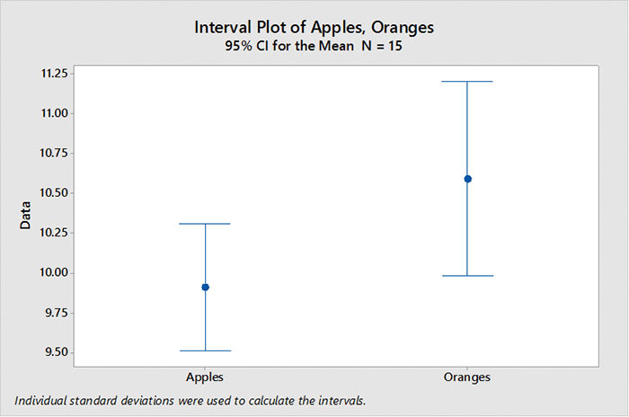
FIGURE 1 is an example of two data sets: “apples” and “oranges.” In the first experiment we had 15 samples of apples and 15 samples of oranges. Plotting the means with their calculated confidence intervals shows we cannot differentiate between apples and oranges. (Since the confidence intervals overlap, we cannot be certain both means are not equal.)

FIGURE 1. Confidence interval, n = 15.
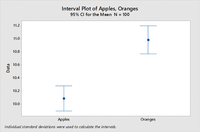
But if we increase the sample size to 100 apples and 100 oranges, our confidence intervals decrease, and we can now tell apples do have lower values than oranges (FIGURE 2).

FIGURE 2. Confidence interval, n = 100. Increasing the sample size decreases the confidence interval.
Capability studies (and Gage R&R studies) use standard deviation as a primary statistic and, like the mean, the standard deviation has a confidence interval.
The confidence interval of the standard deviation is also dependent on the sample size. As the sample size increases, our estimate of standard deviation becomes better. For those who like this stuff, here is the formula for confidence interval on the standard deviation.

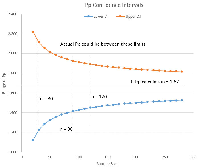
Given a standard deviation of “1” and using the formula above, we can now plot how the confidence intervals contract as sample size increases (FIGURE 3).
In other words, as my capability study’s sample size becomes smaller, the range in which the “true” standard deviation can exist becomes larger.

FIGURE 3. Confidence interval of standard deviation for alpha = 0.05
So, here’s the kicker.
One can calculate the upper and lower limits of Pp for various sample sizes and alpha values and look at the potential range of Pp or Ppk for a capability study.
Let’s look at two examples of how this works.
Example 1: From the chart in Figure 3, let’s assume a sample size of 20 units. Let’s also assume that we ran our capability study and calculated Pp = 1.67.
Now we could stop here and report to our customer that our Pp = 1.67. But, if we do the calculations we see the actual Pp could lie between Pp = 1.12 and Pp = 2.22. If your customer has a savvy Six Sigma expert, you could be busted. In my Six Sigma youth, I was busted. Lately, I’ve been doing the busting. I like that better.
Example 2: If we increase the sample size of the capability study to 120, and if our calculations find a Pp = 1.67, then the actual Pp could be between Pp = 1.45 and Pp = 1.9. With the larger sample size we are much more assured the Pp is actually close to 1.67. In this case, we would have a much better chance of defending a Pp = 1.67.
In summary, never forget that the likelihood the Pp value you report is effectively correct is dependent on the size of the sample. This is one reason to avoid capability studies on small prototype builds and experimental runs.
We can also see from the chart in Figure 3 that once we have a sample size greater than about 90 pieces, the incremental improvement (decrease) in the range of our standard deviation (and thus our Pp) becomes small enough to ignore.
I hope you have enjoyed this series on the vagaries of capability studies (Cp versus Pp, data distribution, and sample size). Practically we cannot always control these factors, but we can at least go into our study with our eyes open and a clear understanding of our “risk of being wrong.”
JOHN BORNEMAN is a Six Sigma Master Black Belt with over 40 years’ experience in electronics manufacturing; This email address is being protected from spambots. You need JavaScript enabled to view it..



 As most readers know, statistical tests calculate a mean and confidence intervals on the mean. We are all familiar with the fact that as our sample size decreases, our knowledge of the “true” mean becomes less and less certain. This is important for tests that use the mean, such as the t-test and ANOVA.