Methods for assessing component temperatures and fan performance.
Cloud technology has become increasingly prevalent, allowing use of 3-D models and numerical methods to analyze CAD models of electronic devices and components. Numerical computations of conduction, convection and radiation are essential for understanding how these heat transfer mechanisms can be utilized for effective cooling techniques.
Advantages of cloud-native simulation include fast and easy access in a web browser, the ability to explore a complete design space and eliminate poor design choices earlier in the development process, and the ability to import geometry without tedious CAD cleanup constraints. The mesh for Immersed Boundary Method (IBM) solvers, for example, is founded on a cartesian grid, making it resilient to geometrical features and obviating CAD simplification. The sheer limitless computing power and scalability of the cloud means sharing simulation capabilities across a full organization of geographically dispersed engineers is simple and easy. Engineers can perform cooling, heat and fluid flow analysis of electronic devices, PCBs, electronics systems and enclosures along with structural and mechanical assessment using a single CAD model, all in one simulation platform.

Figure 1. Joule heating simulation of an electric vehicle inverter showing temperature increase on the bus bars and electric components such as MOSFETs and capacitors.
Thermal Performance of a Raspberry Pi
A Raspberry Pi is simulated using a publicly available 3-D model of the device taken from GrabCAD. A conjugate heat transfer simulation with forced convection (fan) was used to model the computer using standard 30mm fans for cooling. Manufacturer data were used for the fan performance, with four different model types providing data on volumetric flow rate and pressure drop. Simulation tools can determine fan operating points and generate system resistance curves by performing a thermal flow analysis of a Raspberry Pi. Such tools can then be used to determine the system resistance curve and generate a flow rate study to derive the fan operating point, which is done simultaneously.
This approach is instrumental to assess in-situ fan performance in the system or device and optimally cool the heat generation from circuits and components. For the simulation setup, fan inlet and pressure outlet boundary conditions are used, the air is used for the flow region, and several materials are specified for the chips and electronic components, including copper, PCBs, silicon for chips and aluminum for heat sinks (FIGURE 2). Power values represent the CPU (3W) and more minor chips (0.25W). The air inlet is ambient at 19.85°C, and a CSV file is used to upload the fan curve.


Figure 2. Raspberry Pi and a simplified version of the product CAD model for simulation. Images courtesy Michael H. (Laserlicht) / Wikimedia Commons (top) and Ankit Jangid (bottom)
There are several ways (boundary conditions) to specify chip/component temperature or power values:
- Fixed or variable component temperature – a prescribed constant or variable temperature value can be applied to the assigned entities (faces or volumes). This is useful to model constant temperature heat sources or sinks, or to apply a known spatial distribution of temperature.
- Surface heat flux – a prescribed constant or variable heat flux per unit area can be applied to the assigned boundary faces on the geometry model. This is useful to model heat sources or heat sinks, where the power per unit area is known.
- Volumetric heat flux – a power per unit volume is applied to a component, useful when not able to model the component/chip physically.
Likewise, fan performance can be modeled several ways. A boundary condition where the fan inlet is placed can have a direct mass flow applied to it as a velocity inlet with appropriate fluid material properties and ambient temperature. Alternatively, a momentum source can be defined to represent the flow from a fan, and, most recently, engineers can upload fan-curve data in a tabular format directly and use it as a boundary condition. In the case of the Raspberry Pi, we have modeled two fan options (L and H) by taking manufacturer data.
We can visualize heat removal on the chips by looking at surface area average temperatures. FIGURES 3 and 4 show up to 120°C on the CPU (max.). Users can extract point-specific data and pressure drop across air inlets and outlets and assess the chip cooling performance based on comparing multiple fans.

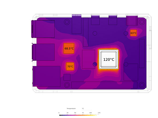
Figure 3. Visualization of temperature on solid domain, showing CPU chip at highest temperature (white/yellow).

Figure 4. Visualization of temperature on solid domain, showing CPU chip at highest temperature (white/yellow).
Fan inlets show a 4.78 pascal (0.5mmAq) pressure difference at a flow rate of 7.55e-4m3/s, and this matches the fan curve data sheet for the baseline model (L). The fan outlets are at 0 gauge pressure as intended. We can easily switch the fan curve data to simulate a more powerful fan (H) for comparison. Doing this shows a 10 pascal (1mmAq) pressure drop, but also a higher achieved flow rate cooling the components. The two are compared in FIGURE 5. Through this analysis, we can start generating a system curve for the enclosure (Raspberry Pi) derived from simulating various fan operating points (orange line in Figure 5). Running 10 simulations of different flow rates in parallel, we generated the entire system curve for the Raspberry Pi in 2 hr. Chip cooling performance based on comparing the two fans is also shown, with the more substantial model H fan better at removing heat (FIGURE 6).

Figure 5. Fan performance curves and Raspberry Pi system resistance curve for different fan models for comparison purposes.

Figure 6. Chip temperature model L vs. model H; H gives lower temp with higher flow rates (CPU).
Heat Flux Across a Resistor
Resistors are used to protect other components in an electric circuit with high voltages or current pulses using highly resistive materials, ideally in a compact structure. The power resistor model in FIGURE 7 has four separate resistive conductor circuits and is used in vehicles to ensure the electronic control unit (ECU) for fuel injection does not overload from high current spikes. The full 12V potential is connected and provides the required high opening current of 22.6A, but the components cannot withstand the high current load for long. The ∼6Ω resistor circuits are added to the circuit with a switch and reduce the current below 2A. The component is mounted at a sheet metal component next to the engine and must only rely on natural convection cooling.

Figure 7. Power resistor device used in the fuel injection circuit in automotive applications.
The electric potential (voltage) gives insights into the voltage drop across electronic components and wires within the electric circuit and the expected voltage drop overall in case of a current drain-driven simulation. The electric current density (A/m2) provides essential information about the electric current flow in the whole circuit and if current density spikes occur. The Joule heat generation (W/m3) result field is used to judge the heat flux that needs to be considered when designing the thermal management solution for the system. Using internal statistical tools, the distributed heat load as well as the integrated total power loss on a part of the model can be extracted.


Figure 8. Joule heating simulation in SimScale, showing a) the electric potential, b) generated heat, and c) current density magnitude on the resistor (red indicates a higher value).
ALEX FISCHER is cofounder and product manager at SimScale (simscale.com) and leads the company's thermal management and electronics solutions; This email address is being protected from spambots. You need JavaScript enabled to view it.. He has a background in computational mechanics and control technology, and has worked for 10 years in a range of product and engineering roles, building a fully cloud and web-based simulation platform.