A review of five useful tools and the basis for using each.

What is the prominent skill process engineers are on the payroll for? It’s their problem-solving skills. Therefore, the process engineer’s function is to solve problems and add value. The better the process engineer becomes at doing this, the more valuable they become. The scientific method is a structured approach to problem-solving that can aid the process engineer in this endeavor.

The scientific method involves looking at the process around you, coming up with an explanation for what you observe, testing your explanation to see if it could be valid, and then either accepting your explanation (for the time being, something better might come along!) or rejecting the explanation and trying to come up with a better one. There are five steps to the scientific method: 1) make observations, develop a theory, 2) propose a hypothesis, 3) design and perform an experiment to test the hypothesis, 4) test your data to determine whether to accept or reject the hypothesis, and 5) if necessary, propose and test a new hypothesis. Let’s define the first four steps in scientific terms.

• Theory – ideas intended to explain what we see and justify a course of action
• Hypothesis – a proposed mechanism of the theory that can be tested
• Experiment – a scientific procedure undertaken to test the hypothesis
• Test – a statistical test used to determine the plausibility of the hypothesis.

Statistics is a branch of mathematics that deals with collecting, analyzing, interpreting and presenting numerical data. Statistics is not merely the science of analyzing data, but the art and science of collecting and analyzing data. Statistics are only tools to help us; they do not replace the process engineer’s skill and intelligence. Statistics use hypotheses, experiments and hypothesis testing.

With hypothesis, there is a null (H0) and an alternative (H1). In general, the null hypothesis is a statement that two population means are equal. In general, the alternative hypothesis is a statement that two population means are not equal. Formally, the null and alternative hypotheses are written as:

H0 : µ1 = µ2
H1: µ1 ≠ µ2

With hypothesis testing, in colloquial terms, we either accept the null hypothesis or accept the alternative hypothesis based on a probability value (p-value). Probability is a branch of mathematics that deals with the occurrence of a random event. P-values are expressed from zero to one and are the probability of an event having occurred. The general interpretation of p-values is as follows:

• < 0.05 are statistically significant
• 0.05 ≤ p-value ≤ 0.10 may have a practical difference
• 0.10 are generally considered non-significant

Statistically significant means that the results in the data are not likely explainable by chance alone. Practical difference requires the process engineer to logically determine if the population mean differences have any practical value. Non-significant means the results in the data lie within the limits of chance.

There are five practical statistical tools the process engineer should be familiar with. These five tools are the Bland-Altman Plot, Tukey End Count, Mann-Kendall Trend, Bayesian Inference Box, and the Reliability by Confidence (R by C) Table. These five statistical tools can answer such questions as: How close do two different measurement devices agree on measurements? Do these data samples have the same distributions? Is there a trend in the data? How can I conduct a simple experiment and data analysis? How do I interpret test data in the context of reliability?

The Bland-Altman Plot is used to visualize the measurement differences between two instruments.¹ The plot is helpful for determining two things: What is the average difference in measurements between the two instruments? What is the typical range of agreement between the two instruments? The plots have the following three lines: The average difference in measurements between the two instruments, or “bias”; the 95% upper confidence limit for the average difference, or “limit of agreement”; and the 95% lower confidence limit for the average difference, or “limits of agreement.”

In general, 95% of the differences between the two instruments fall within the limits. Whether to accept that the two instruments agree depends on the level of precision needed in a particular domain. For example, the process engineer measures the same 10 pads from various PCBs plated with electroless nickel immersion gold (ENIG) on two different XRF machines. The process engineer is interested in the gold thicknesses (TABLE 1).

Table 1. Gold Measurements (microinches)

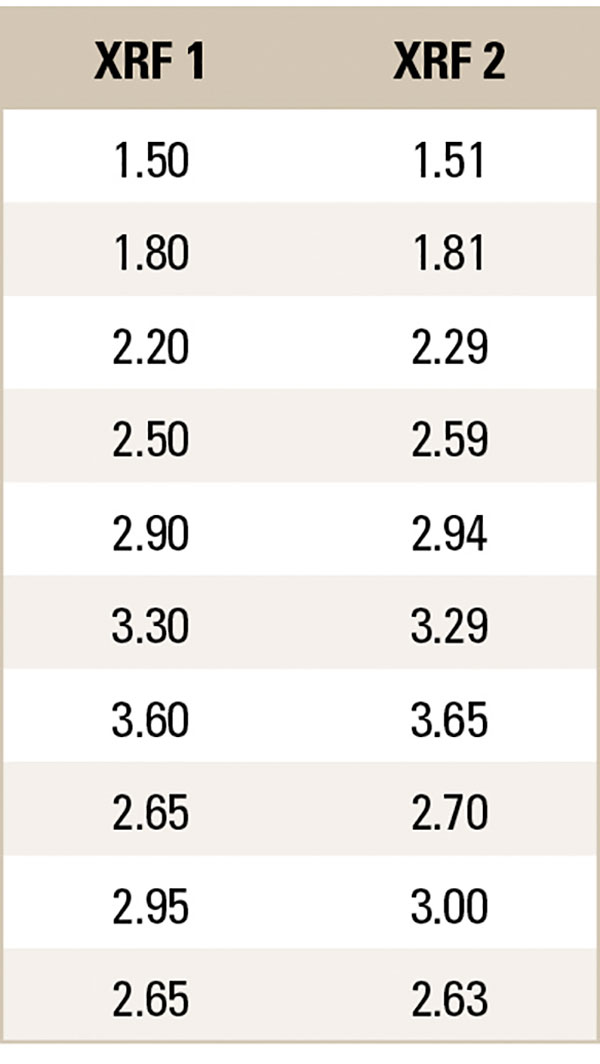
The process engineer plots the data on a Bland-Altman Plot (FIGURE 1). The average difference between XRF measurements is -0.04 microinches, and the absolute range of agreement is 0.15 microinches. These values are reasonable. The process engineer concludes to accept that the two instruments agree.

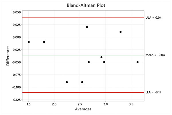
Figure 1. Bland-Altman plot.

The Tukey End Count is a nonparametric hypothesis test that compares two independent sample medians.² Each independent sample size needs to be n ≥ 5. The two datasets are ordered, and a count of the number of nonoverlapping points (end count) is used to determine if the samples have different medians. An end count of ≥ 7 provides 95% confidence there is a statistical difference. The end count test does not work on all problems; if one sample contains both the highest and lowest values, there is no end count. For example, the process engineer gathers etch rate data from two shifts. The process engineer is interested if the first and second shifts are statistically etching the same amount of copper (TABLE 2).

Table 2. Etch Rate Measurements (microinches)

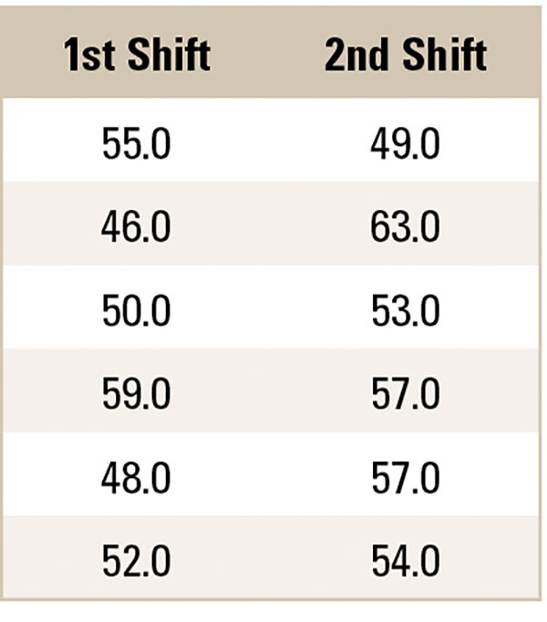
The process engineer plots the data on a dot plot (FIGURE 2). The number of nonoverlapping points on the left is two, and the number of nonoverlapping points on the right is one. The end count is 2 + 1 = 3, which is < 7. The process engineer concludes there is no statistical difference in etching between first and second shifts.

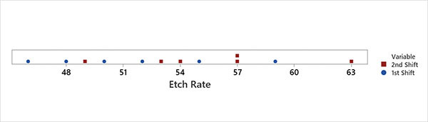
Figure 2. Dot plot of Tukey End Count.

The Mann-Kendall Trend test is a nonparametric hypothesis test for trends.³ The data are arranged in chronological order, compared pairwise, and coded “+” or “-” depending on whether the preceding number is greater or less than the postceding number. The test involves computing a statistic, S, which is the difference between the number of pairwise differences (“+” or “-”) that are positive minus the number that are negative. If S is a large positive value, then there is evidence of an increasing trend in the data. If S is a large negative value, there is evidence of a decreasing trend in the data. The null hypothesis is that there is no trend in the data values.

For example, the process engineer gathers daily process yield data for the past 10 days. The process engineer is interested if there is a trend in the yield data (TABLE 3).

Table 3. Process Yield Data

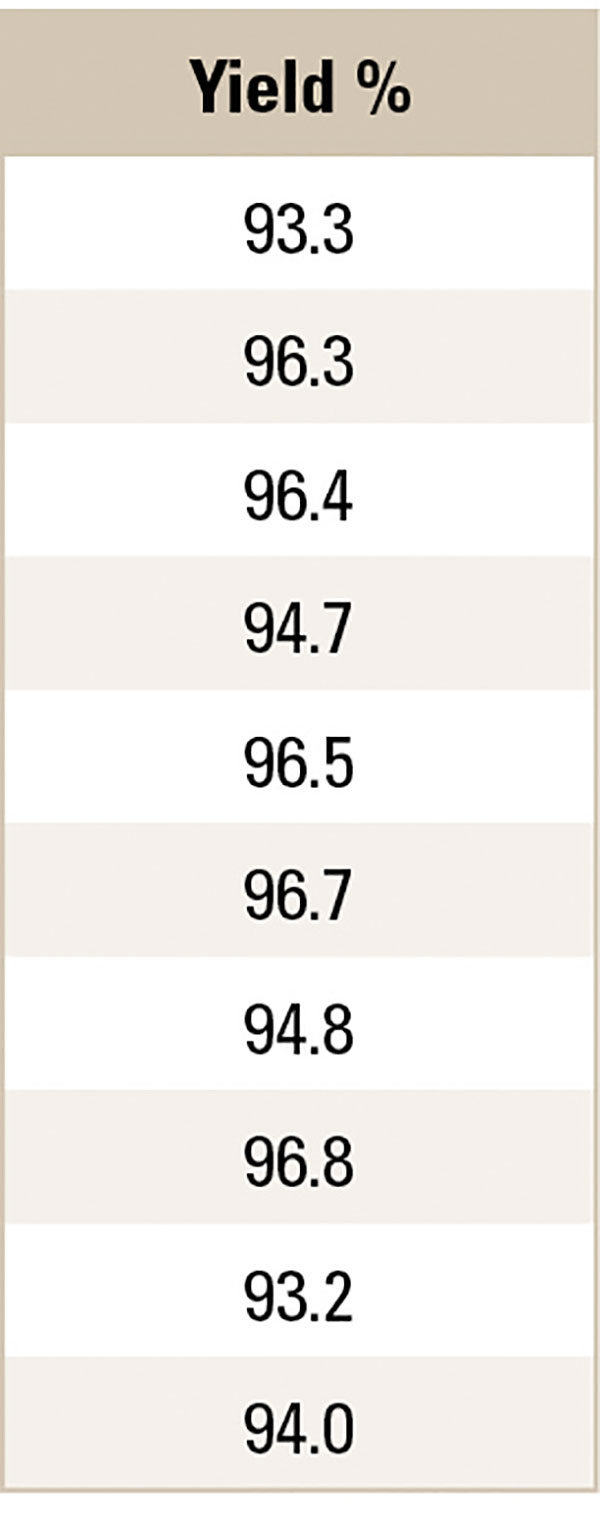
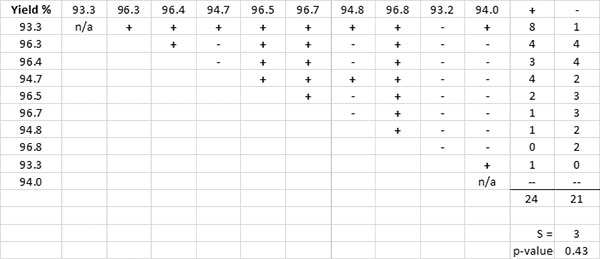
The process engineer computes the pairwise difference (TABLE 4). The computed S statistic is 3, with a corresponding p-value of 0.43, which is significantly above 0.05. The process engineer concludes there is no statistical trend in the yield data.

Table 4. Yield Data Pairwise Differences

The Bayesian Inference Box is based on Bayes’ theorem, which deals with sequential events.⁴ When new information is obtained for a subsequent event, that new information is used to revise the probability of the initial event. Bayes’ theorem uses conditional probability. We use P(B|A) to denote the conditional probability of event B occurring, given that event A has already occurred. There are three sections of a Bayesian Inference Box.

Prior: Describes how sure we are that each hypothesis is true. Note: Two or more hypotheses can be tested, and they all must sum to 1.

Likelihood: Imagine each hypothesis is true and ask: “What is the probability of getting the data that I observed?” Note: The likelihood does not need to sum to 100.

Posterior: How confident are we that hypothesis “H” is true, given that we have observed data “D?”

For example, the process engineer reviews a cross-section of an ENEPIG-plated printed circuit board with a potential nickel hyper-corrosion defect (FIGURE 3). The process engineer builds a Bayesian Inference Box with two hypotheses (H1 and H2) and assigns prior probabilities (0.80 and 0.20) based on their experience. The process engineer knows that nickel hyper-corrosion enriches the percent phosphorous in the defect area, so the process engineer collects scanning electron microscope-energy dispersive spectroscopy (SEM-EDS) data on the bulk percent phosphorous in the defect area and a normal nickel deposit area. The process engineer imagines each hypothesis is true and asks: “What is the probability of getting the data that I observed?” They then assign a likelihood (95 and 4) based on the observed data. The process engineer calculates the posterior and concludes with 99% confidence there is nickel hyper-corrosion (TABLE 5).

Table 5. Bayesian Inference Box

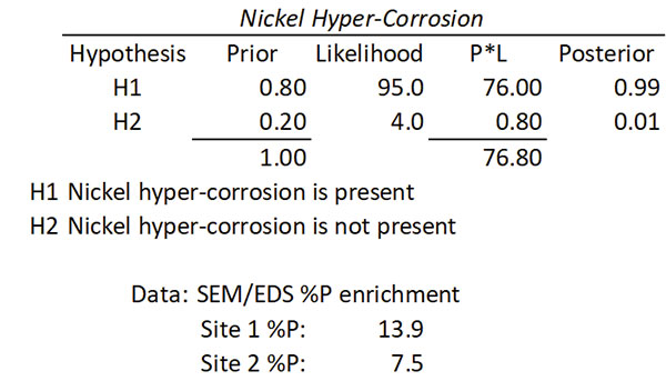
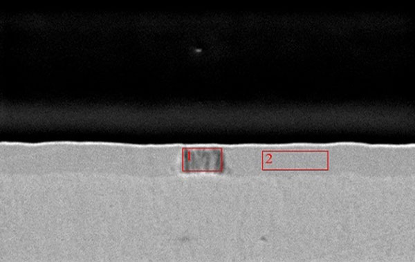
Figure 3. Potential hyper-corrosion defect.

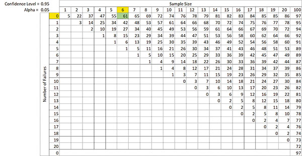
The Reliability by Confidence Table provides valuable information about sample size and uncertainty.⁵ The R by C notation signifies what reliability requirement (R) at time (t) we want to meet with a level of confidence (C). An R95C95 means a 95% probability of survival, R(t), with 95% confidence in achieving that requirement. R(t) is viewed as a lower confidence limit on reliability, denoted as RL. For example, the process engineer thermal cycles six parts for 200 cycles with zero failures. Sample size is n = 6, with 0 failures, R by C = 61. Interpretation: We are 95% confident the probability of survival at 200 cycles is at least 61% (R61C95), or we are 95% confident the failure rate at 200 cycles is no more than 39% (100% - 61% = 39%) (TABLE 6).

Table 6. Reliability by Confidence Table

Conclusions

The process engineer’s function is to solve problems and add value. The scientific method is a structured approach to problem-solving that can aid the process engineer in this endeavor. Statistics are powerful tools. Choosing, using and interpreting the proper statistical tool is critical for the process engineer. There are five practical statistical tools the process engineer should be familiar with. These five tools are the Bland-Altman Plot, Tukey End Count test, Mann-Kendall Trend test, Bayesian Inference Box and the Reliability by Confidence (R by C) Table. •

References

1. J. M. Bland and D. G. Altman, “Statistical Methods for Assessing Agreement between Two Methods of Clinical Measurement, Lancet, 8;1(8476):307-10, 1986.
2. J. W. Tukey, “A Quick, Compact, Two-Sample Test to Duckworth’s Specifications,” Technometrics, vol. 1, no. 1, February 1959.
3. US Environmental Protection Agency, “Data Quality Assessment: Statistical Methods for Practitioners EPA QA/G-9S,” 2006.
4. T.M. Donovan, and R.M. Mickey, Bayesian Statistics for Beginners: A Step-By-Step Approach – Illustrated Edition, Oxford University Press, 2019.
5. G. Wasserman, Ph.D., Reliability Verification, Testing, and Analysis in Engineering Design, Marcel Dekker, 2003.

Patrick Valentine, Ph.D., is technical and Lean Six Sigma manager at Uyemura USA (uyemura.com); This email address is being protected from spambots. You need JavaScript enabled to view it.. He holds a doctorate in Quality Systems Management from New England College of Business and ASQ certifications as a Six Sigma Black Belt and Reliability Engineer.

• Prev
• Next