An incomplete picture can “mask” significant issues.
Measurement system analysis (MSA) evaluates the overall capability of a measurement system. Measurement capability serves as a foundational element for ensuring product quality, as reliable measurements are essential for maintaining consistency and meeting specifications. Before any measurement system can operate in production, a thorough evaluation determines its capability. This assessment ensures the system provides accurate and precise measurements, laying the groundwork for robust quality control practices.
A capable measurement system should be both precise and accurate. Precision refers to the variability of the gauge, focusing on how close the measurements are to each other when repeat measurements are taken. When determining the precision of a measurement system, consider repeatability and reproducibility. Accuracy refers to how closely a measured value aligns with a standard or reference value. Many tools evaluate the MSA of a process.
The Type 1 gauge study is a common starting point in a comprehensive MSA program. This study involves repeated measurements of a single sample using one gauge and one operator. It provides insights into both the gauge’s accuracy by comparing results to a reference value and its precision through the consistency of repeated measurements. In industry, professionals commonly select a reference value standard in the center of the measurement range and typically utilize a NIST traceable standard. Operators generally take 30 measurements and evaluate the capability indices (Cg and Cgk). If the gauge achieves a minimum capability index of 1.00, it is deemed acceptable. A comprehensive MSA program goes beyond this initial evaluation, however, offering a more thorough and reliable assessment of the measurement system’s capability.
A comprehensive MSA program is essential for complex processes in printed circuit board manufacturing, particularly for surface finishes such as electroless nickel immersion gold (ENIG). While a Type 1 gauge study is a useful starting point for evaluating a measurement system, it has limitations. The study evaluates the gauge’s performance at a single point and fails to account for variability across a range of values. For processes requiring measurements over a range of thicknesses or parameters, this limited focus may overlook variability in accuracy (bias) and precision (repeatability) that can occur at different points within the range. To ensure a robust measurement system, additional statistical studies are needed to assess performance across the entire operating range.
In manufacturing, these measurement system challenges increase the risks of Type 1 and Type 2 errors, which influence scrap and quality outcomes. A Type 1 error (false positive) occurs when a good part is mistakenly rejected as defective, leading to unnecessary scrap or rework. On the other hand, a Type 2 error (false negative) happens when a defective part is wrongly accepted as good, which can result in quality issues downstream or with customers. Minimizing these errors is critical for reducing waste and ensuring product reliability. The gauge’s bias and linearity need to be evaluated to avoid these risks.
Performing a bias and linearity study (B&L) is crucial in avoiding Type 1 and Type 2 errors. Bias refers to the difference between the average measurement and the known standard being measured. Linearity indicates how bias varies throughout the gauge’s application range. The B&L study plays a significant role in identifying and addressing these issues, enhancing the reliability of the MSA process, reducing measurement uncertainties and improving overall quality control.1,2
Methods and Materials
To run a bias and linearity gauge study, select a minimum of five representative parts across the measurement range of the gauge. Ensure each reference part has a known measurement value and collectively represents the full range of actual or expected measurements. Use NIST-traceable reference values. One operator should perform all the measurements, conducting at least five per reference part, and collect the data at random. Determine measurement times based on the smallest measurement time required to reach acceptable Cg and Cgk values on a Type I Gauge study. After taking the measurements, perform a statistical analysis.3
To analyze the bias and linearity of the gauge, start by looking at the fitted regression line on the bias versus reference value plot. Fit a regression line to the bias values using ordinary least squares regression.4 Ideally, the plot will have a horizontal line through the values indicating that the bias does not change across the reference parts and the measurement system bias is negligible. If the plotted line is sloped, linearity is an issue, and the gauge linearity needs to be evaluated. Generally, the closer the slope of the fitted line is to zero, the better the gauge linearity.
Once this visual check is complete, evaluate the gauge linearity using the p-value for the slope of the fitted line. If the p-value is greater than 0.05, linearity is not present, and assessment of the system’s bias should continue. A p-value less than or equal to 0.05 indicates an issue with linearity. In this case, it is impossible to assess the gauge’s overall bias. Instead, interpret the p-values for the individual reference values only.3
After evaluating linearity, assess the bias of the measurement system. In an ideal scenario, the bias should remain consistent throughout the application range. A positive bias indicates the gauge measures high, while a negative bias indicates the gauge is measuring low. If linearity is not present, use the p-values to interpret the overall bias. For each reference value, if the p-value is greater than 0.05, conclude that the bias equals zero. For the average bias, if the p-value is greater than 0.05, conclude that the average bias is equal to zero. If the p-value is less than or equal to 0.05, conclude that the bias is not equal to zero.3 This may indicate a problem with the reference standard, a systematic problem in the equipment, or a faulty measurement procedure. A solid understanding of the process is important to determine whether the statistically significant bias is also a practical difference.
Example
Using an ENIG calibration program, an example was performed to assess the measurement capability of a Bowman K-series x-ray fluorescence (XRF) unit. The XRF was calibrated using three ENIG standards with gold thicknesses of 1.02µin, 2.51µin and 4.09µin to encompass the entire gold range as defined in IPC-4552B.5 After calibration, a Type 1 gauge study was completed using the 2.51µin standard by taking 30 measurements at 30 sec. (Figure 1). The Type 1 gauge study yielded acceptable capability indices with a Cg value of 5.77 and a Cgk value of 5.75. Following IPC-4552B, the XRF unit would be considered capable.5

Figure 1. Type 1 gauge study.
A B&L study was completed (Figure 2) to further assess the capability of the gauge. The B&L study was initially performed with eight reference samples with gold thicknesses between 1.5 and 3.6µin. These thicknesses were selected to best represent the gold thickness range as stated in IPC-4552B.5 The p-value for the slope was 0.106, greater than 0.05, indicating issues with linearity were not present. The p-value for the bias was 0.000, less than 0.05, indicating the bias is not equal to zero. While statistically significant, the bias value of 0.07 is not practically significant. This gauge would be considered capable of the IPC-4552B gold thickness range.

Figure 2. B&L study eight reference parts.
Additional reference samples were selected at 4.1µin and 6.0µin, as shown in Figure 3, to evaluate the performance of the XRF system beyond the standard industry gold thickness range. While IPC-4552B typically defines acceptable ENIG thicknesses for nickel and gold, production often sees parts exceeding this range due to customer requirements or process drift. The gauge’s bias and linearity in each case were assessed by testing parts outside this window, where process monitoring and measurement accuracy are critical.

Figure 3. B&L Study 10 reference parts.
This study revealed a linearity issue at the range’s extremes, with the bias’s slope versus reference value plot deviating significantly from zero (p-value less than 0.05). There is a statistical and practical bias of approximately 0.5µin once operating outside the IPC-4552B range. This suggests that the measurement system’s accuracy remains inconsistent across the full operating range. These deviations can misclassify parts. For example, if bias causes a conforming product to appear nonconforming, operators may face unnecessary rework or scrap. Conversely, if the gauge underestimates thickness in critical areas, a defective part may be accepted and released to the customer. These measurement errors undermine product quality, increase operating costs, and damage customer relationships.
When only a limited number of standards focus on the nominal value or the center of the range, the measurement system’s behavior at the upper and lower ends can go uncharacterized, as seen in this example. This incomplete picture can mask significant issues such as inconsistent bias across the range or a lack of linearity in certain regions. The gauge capability becomes more representative of the whole process by selecting standards that encompass the entire measurement range. This approach supports more accurate statistical analysis, narrows confidence intervals and improves the detection of systematic error. The Measurement Systems Analysis Reference Manual, published by the Automotive Industry Action Group, recommends evaluating measurement systems across their full operational range to ensure reliable data and trustworthy decision-making.6
Conclusion
Incorporating a bias and linearity study into the current MSA process significantly enhances gauge capability and supports the pursuit of world-class quality. Performing a full measurement system analysis that includes bias and linearity studies verifies data throughout the production process. This verification eliminates the false sense of measurement reliability that introduces process risk and prevents accurate root cause analysis. Engineers might respond to what they believe are real trends or issues when acting on flawed data.4 In the worst-case scenario, defective products may reach the customer, leading to field failures, warranty claims, or brand erosion. These consequences become especially critical in industries that rely on high-reliability electronics.
References
- Abdelgadir, C. Gerling and J. Dobson, “Variable Data Measurement Systems Analysis: Advances in Gage Bias and Linearity Referencing and Acceptability,” International Journal of Metrology and Quality Engineering, November 2020.
- Simion, Assessing Bias and Linearity of a Measurement System, 2015.
- C. Montgomery, Introduction to Statistical Quality Control, 7th ed., Wiley, 2017.
- J. Wheeler, EMP III: Evaluating the Measurement Process & Using Imperfect Data, 2006.
- IPC, IPC-4552B, “Specification for Electroless Nickel/Immersion Gold (ENIG) Plating for Printed Circuit Boards,” April 2021.
- Automotive Industry Action Group (AIAG), Measurement Systems Analysis (MSA) Reference Manual, 4th ed., 2010.
Acknowledgement
The authors would like to acknowledge Bowman XRF for their generous support in providing access to their instrumentation and assisting with data collection. The use of the Bowman K-series XRF was instrumental in conducting our measurement system analysis.
April Labonte is North American technical manager for Uyemura USA (uyemura.com); This email address is being protected from spambots. You need JavaScript enabled to view it.. She holds a bachelor’s in chemical engineering from the University of California San Diego. Brittany Malin is laboratory & continuous improvement manager, Uyemura USA; This email address is being protected from spambots. You need JavaScript enabled to view it.. She holds a bachelor’s in chemistry and mathematics from Central Connecticut State University and ASQ certifications as a Six Sigma Black Belt and Reliability Engineer.