Using the Weibull distribution to model gold wire bonding on ENEPIG.
The most used distribution in reliability analysis may be the Weibull distribution. Its genesis can be traced back to Waloddi Weibull’s invention in 1937. Then, in 1951, Waloddi presented his hallmark paper to the American Society of Mechanical Engineers (ASME) on this subject, claiming that his distribution applied to a wide range of problems. He showed several examples, ranging from the fiber strength of cotton to the fatigue life of steel.1
The Weibull distribution is versatile and fairly easy to interpret. It can be used to model a wide range of applications in engineering, medical research, quality control and finance. For example, the distribution is frequently used with reliability analyses to model time-to-failure data. It is also used to model skewed process data in capability analysis.
The Weibull distribution may not always provide the best fit for a data set. It may not work as effectively for product failures caused by chemical reactions or degradation; e.g., corrosion. These situations can occur with semiconductor failures. Usually, in these types of situations, the lognormal distribution is used.
2 (or 3) Parameters
The Weibull distribution is described by its shape, scale and threshold parameters. The simplest Weibull distribution has two parameters: the shape or beta (β) parameter and the scale or eta (η) parameter. This simpler Weibull distribution is known as the two-parameter Weibull distribution. The more complex Weibull distribution has three parameters: the shape or beta (β) parameter, the scale or eta (η) parameter, and the threshold parameter. Adding the threshold parameter changes the nomenclature to the three-parameter Weibull distribution.
The optional third parameter, the threshold parameter, can be set to any value to move the lower bound. The threshold parameter default set point is zero because we can’t have failures without first applying stress to the test items. Therefore, the Weibull distribution is bounded on the left tail, not taking on a value below zero. The Weibull distribution can take various forms depending on the parameters’ values. A look at the three parameters:
Shape or beta (β): This describes how the data are distributed and determines the shape of the Weibull distribution. A shape of three approximates a normal distribution curve. A low value, say one, gives a right-skewed curve. A high value, say 10, gives a left-skewed curve (Figure 1).

Figure 1. Weibull shape (beta) parameter.
Scale or eta (η): Determines the spread of the Weibull distribution by defining the position of the Weibull curve relative to the threshold. A larger scale value stretches the distribution, while a smaller scale value squeezes the distribution. For the Weibull distribution, the scale is always the 63.21 percentile of the distribution of possible values. For example, a scale of 15 indicates that 63.21% of the parts will fail in the first 15 units of stress (e.g., hours, cycles, grams, etc.) after the threshold time (Figure 2).
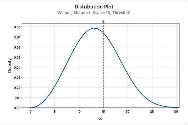
Figure 2. Weibull scale (eta) parameter.
Threshold: A fixed characteristic of the population distribution that provides a parameter of the earliest possible failure time. The threshold parameter describes the shift of the distribution away from zero. All data must be greater than the threshold parameter. The two-parameter Weibull distribution is the same as the three-parameter Weibull with a threshold of zero. For example, the three-parameter Weibull (3,75,40) has the same shape and spread as the two-parameter Weibull (3,75) but is shifted 40 units to the right (Figure 3).
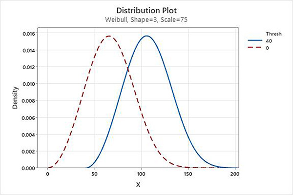
Figure 3. Weibull threshold parameter.
Because of its versatility, the Weibull distribution can model all three stages of a product’s life cycle: infant mortality, design life, and wear-out. The Weibull “bathtub curve” is a conceptual model for describing reliability-related phenomena at the component level over a product’s life cycle (Figure 4). Each life cycle stage is defined below.
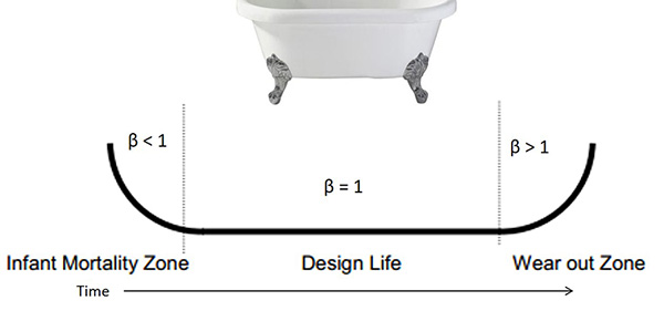
Figure 4. Bathtub curve with its three life cycle stages.
Infant mortality (β < 1): Failures that occur early during reliability testing are caused by manufacturing defects such as poor quality, out-of-spec processing, substandard manufacturing and assembly practices, etc.
Design life (β = 1): A constant failure rate (a constant percentage fails among those units still “alive”) with random failures (independent of time) due to excessively high loads, environmentally induced stresses, etc.
Wear-out, early (1 < β < 4): Early wear-out begins with failures of weaker items and progresses to wear-out of stronger parts as β moves from one to four. Failures occur due to low cycle fatigue, corrosion, aging, friction, etc.
Wear-out, rapid (β > 4): These are highly reliable products, but failures occur due to fatigue, corrosion, aging, friction, etc.
It is easy to see how these three parameters can be manipulated to fit various problems, just as Waloddi Weibull stated in 1951.1 The primary advantage of Weibull analysis is the ability to provide reasonably precise failure analysis and time-to-fail forecasts with extremely small sample sizes.2
Parameter Interpretation
The interpretation of the shape (β) and scale (η) parameters must be taken in reference to the desired reliability of the parts and their design life. Large shapes (β) within the design life are a source of concern as there is a risk of the entire population failing quickly as the parts age into the wear-out part of the life cycle. On the other hand, if the Weibull scale value (η) is well beyond the minimal desired design life, the probability of failure before part retirement is negligible. Large shapes (β) are a source of happiness in this case. Most large shapes (β) have a safe period before the onset of failures, where the probability of failure is negligible. The larger the shape (β) for a given scale (η) value, the smaller the variation in times to failure and the more predictable the results of the product (tighter manufacturing controls). A vertical shape (β) of infinity implies perfect design, manufacturing and quality control.2
Assessing the Weibull Plot Fit
Three typical goodness-of-fit measures are used to assess the fit:
Anderson-Darling (AD) adjusted statistic: A relative goodness-of-fit measure for the selected distribution that can be used to compare its fit to the data provided by alternate distributions. One can compare the AD statistic for several distributions with the same number of parameters; smaller AD values indicate a better fit. To conclude that one distribution is the best, however, its AD statistic must be substantially lower than the others. When the AD statistics are close together, use the probability plots to choose among them.3,4,5
Correlation coefficient (Pearson’s): Measures the strength of the linear relationship between the data set and the chosen distribution. Suppose the distribution fits the data well when plotting points on a probability plot graph. In that case, these points will fall almost on a straight line (superimposed on, or very close to, the diagonal line), and the correlation coefficient will approach one. This statistic’s maximum value is one. The idea of a probability plot correlation coefficient came from James Filliben, who also discussed extensions of the test for non-normal distributional hypotheses.6 Vogel completed additional probability plot correlation coefficient work on several distributions.7
Visual examination – probability plot for fit and competing failure modes: The data points (failure times) should line up close to a diagonal line, indicating a good fit. The origin of the blue diagonal line comes from the shape (β) and scale (η) parameters iteratively estimated from the data set and plotted. The percent (y-axis) follows the shape (β) parameter, with the scale (η) at the 63.21% percentile (Figure 5).
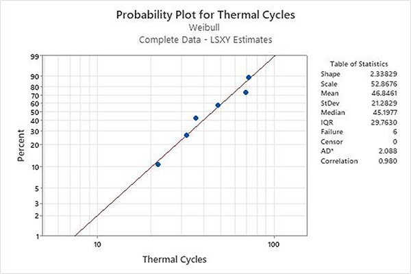
Figure 5. Weibull probability plot fit.
The plotted data in Figure 5 have an excellent fit with a correlation coefficient of 0.980. The Anderson-Darling (AD) statistic is relative. Still, it would be of significant value if we compared the Weibull distribution with, say, the lognormal distribution. Then, whichever distribution had a significantly smaller AD statistic would indicate a better fit. During visual analysis, one needs to look for competing failure modes; e.g., dog legs, cusps, and corners, as these indicate two or more competing failure modes present (Figure 6). It is generally best practice to analyze multiple failure modes separately when they behave differently.
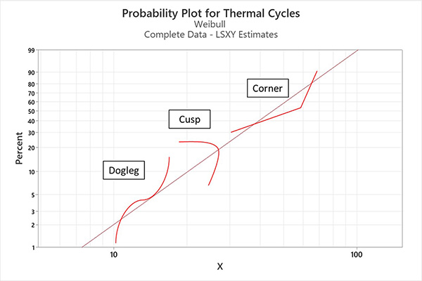
Figure 6. Competing failure modes. Note: for illustrative purposes only; some patterns may not be mathematically possible.
Reliability Testing
Probability is a branch of mathematics that deals with the occurrence of a random event. P-values are expressed from zero to one and are the probability of an event having occurred or occurring in the future. Reliability is the probability (0 ~ 1) of a product performing its intended function over its specified usage period and under specified operating conditions that meet or exceed customer expectations. Reliability is simply quality over time.
Reliability theory developed apart from the mainstream of probability and statistics. It was used primarily as a tool to help nineteenth-century maritime and life insurance companies compute profitable rates to charge their customers.3 In today’s technological world, nearly everyone depends upon the continued functioning of complex machinery and equipment.3
In reliability testing and analysis, any time there are actual failures, either with or without censored data, we use an empirical distribution for analysis and inference about the population. An empirical distribution is the distribution function associated with the actual measure of a sample.
Censored data means we do not know exact failure times (e.g., the reliability testing was stopped before a failure occurred). We call this “right” censored data. The data value is coded; “0” is usually used for censored values, and “1” is used for actual failure times.
A Worked Example
Electroless nickel electroless palladium immersion gold (ENEPIG) is a standard printed circuit board final finish. The electroless palladium layer provides a base for gold wire bonding. The ENEPIG process engineer is qualifying their new final finish line. The process engineer will evaluate 1-mil gold wire bonding (ball and stitch) as part of the qualification. The process engineer plates samples under controlled conditions and collects wire bond pull data (Table 1). The process engineer creates a Weibull probability plot and assesses the fit (Figure 7).
Table 1. 1-mil Gold Wire Bond Pull Data
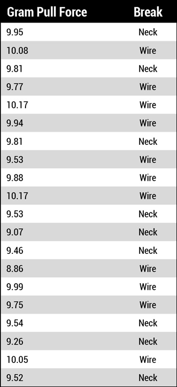
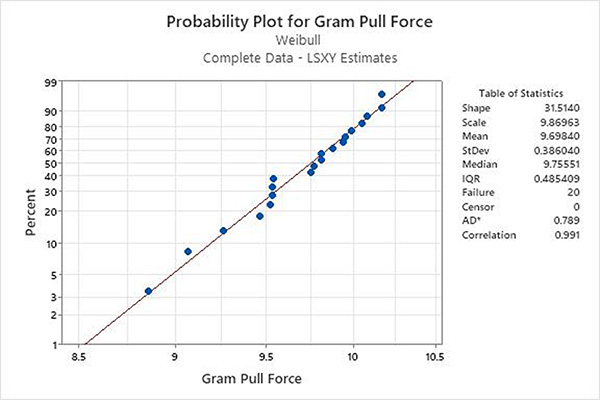
Figure 7. Weibull probability plot.
The plotted data in Figure 7 have an excellent fit with a correlation coefficient of 0.991. The Anderson-Darling (AD) statistic is relative. Still, it would be of significant value if we compared the Weibull distribution with, say, the lognormal distribution. During visual analysis, the process engineer looks for competing failure modes (dog legs, cusps and corners), but none exist. The data points (failure times) line up close to a diagonal line, indicating a good fit. The process engineer reviews and is satisfied with the fit. Next, the process engineer begins to interpret the shape (β) and scale (η) parameters in reference to the desired reliability of the parts and their design life.
The shape parameter is 31.5 (rapid wear-out), the scale parameter is 9.86 (grams), and the threshold parameter is zero (a two-parameter Weibull distribution). The process engineer references MIL-STD-883K Condition D with 1-mil gold wire, pre-seal, which requires a minimum bond force of 3g.8 The Weibull scale value of 9.86g is well beyond the minimal desired reliability of 3g, so there is a negligible probability of failure before part retirement. In this case, the enormous shape value of 31.5 is a source of happiness due to the smaller variation in gram pull forces. In other words, the results of the ENEPIG and the wire bonding processes are more predictable due to tighter manufacturing controls. Last, for ease of interpretation, the process engineer creates a Weibull probability distribution plot using the shape parameter of 31.5 and the scale parameter of 9.86 (Figure 8).
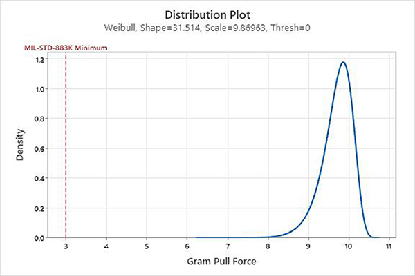
Figure 8. Weibull probability distribution plot.
Conclusions
The genesis of the Weibull distribution can be traced back to 1937. It is a versatile distribution that can be used to model various applications in engineering, medical research, quality control, and finance. The Weibull distribution is described by its shape, scale and threshold parameters. Because of its versatility, the Weibull distribution can model all three stages of a product’s life cycle: infant mortality, design life, and wear-out stages. Three typical goodness-of-fit measures are used to assess the Weibull fit: the Anderson-Darling statistic, the correlation coefficient (Pearson’s), and a visual examination of the probability plot. In today’s technological world, nearly everyone depends upon the continued functioning of complex machinery and equipment. Reliability is simply quality over time.
References
- Weibull, “A Statistical Distribution Function of Wide Applicability,” ASME Applied Journal of Mechanics, pp. 293-297, 1951.
- Robert B. Abernethy, The New Weibull Handbook 5th Ed,
3. NIST Engineering Statistics Handbook, 2012. https://www.itl.nist.gov/div898/handbook/
- Ryan, Modern Engineering Statistics, 2007.
- Gary, S. Wasserman, Reliability Verification, Testing, and Analysis in Engineering Design, 2003.
- James, J. Filliben, “The Probability Plot Correlation Coefficient Test for Normality,” Technometrics, vol. 17, no. 1, pp. 111-117, 1975.
- Richard, M. Vogal, “The Probability Plot Correlation Coefficient Test for the Normal, Lognormal, and Gumbel Distributional Hypotheses,” Water Resources Research, vol. 22, no. 4, pp. 587-590, 1986.
- MIL-STD-883K, 2017.
Patrick Valentine is technical and Lean Six Sigma manager for Uyemura USA (uyemura.com); This email address is being protected from spambots. You need JavaScript enabled to view it.. He holds a doctorate in Quality Systems Management from Cambridge College, a Six Sigma Master Black Belt certification from Arizona State University, and ASQ certifications as a Six Sigma Black Belt and Reliability Engineer.