Despite different approaches and different coding, the results were remarkably close.
In this paper, we evaluate different simulation tools and compare how well they describe the transmission line properties. This involves extracting some of the important parameters such as characteristic impedance (z0), time delay (td), dielectric constant (dk), near-end crosstalk (s31), far-end crosstalk (s41) and transmission coefficient (S21). A differential pair structure for microstrip and stripline was built with the lines in edge-coupled formation. Simulations were performed for both tightly and loosely coupled cases. For the purpose of comparing how well the simulation tools describe the transmission line properties, a number of EDA tools were used, such as Advanced Design System (ADS), Mentor Graphics HyperLynx, Polar Instruments Si9000e, etc. All use a different method of solving for the fields and calculation of Scattering-parameters. The motive behind performing these simulations was to analyze how a few important figure-of-merits can be extracted from a 4-port S-parameter simulation.
An essential element in circuit board design is engineering the stackup to achieve specific transmission line properties, like characteristic impedance and crosstalk. The best tool for this is a field solver, either a 2D or 3D. But with so many commercially available, the question is always which one to use. Every commercial tool vendor says their tool is accurate. If this is the case, then when analyzing the same geometry, they should return the same result.
In this study we evaluated the relative precision of a few commercial field solver tools and compared their predictions. We cannot address the question of absolute accuracy in this analysis, only the relative comparison between them.
Structures analyzed. Two different geometries were analyzed: differential microstrip and stripline, both loosely coupled and tightly coupled. Since the tightly coupled case is the most sensitive test of the field solver results, only this case will be reported here.
In each pair, the line width was set at 5 mils for 0.5 oz. copper and an edge-to-edge separation of 5 mils. For this initial study, the lines were engineered lossless. The dissipation factor was set to 0, and the copper conductivity was set to 1×1050 S/m. A summary of the cross-section details is shown in FIGURE 1 and TABLE 1.

Figure 1. Cross-section images.
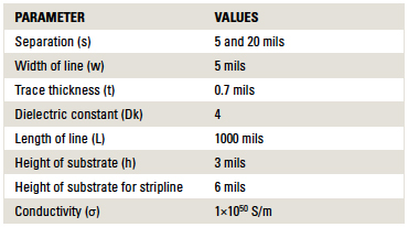
Table 1. Stackup Design for SL and MS Differential Pair and Parameters Used
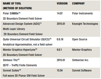
Tools evaluated. A total of six different field solver tools were evaluated. These were picked based on being readily available. No endorsement or recommendation on a “best” tool is made here. All we can do in this study is compare the tools, not offer a statement of “goodness.”
In TABLE 2, we list the six tools used in this study. Their output in each case is an S-parameter file in touchstone format, which describes the 4-port S-parameters of a differential pair, 1" long. In each case, the port impedance was 50Ω.
Table 2. EDA Tools Used
Analysis of the S-Parameters
Each tool calculates the frequency-dependent S-parameters from 10MHz to 20GHz in 10MHz steps. Rather than just compare all 16 of the S-parameter elements, we decided to extract from each S-parameter file a few relevant figures of merit for each differential pair structure.
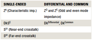
In particular, the four most important terms for two coupled, single-ended transmission lines are the characteristic impedance, the effective dielectric constant, the near-end crosstalk coefficient and far-end crosstalk coefficient.
When these two single-ended lines are considered as one differential pair, then we can describe them in terms of the even and odd mode impedances and the even and odd mode or differential and common effective dielectric constant.
These eight figures of merit are summarized in TABLE 3.
Table 3. Important Figures of Merit
From S-Parameters to Figures of Merit
Each of the 4-port S-parameter files contained about 16 x 2 x 2000 = 64,000 different numbers. None of these specific numbers is the characteristic impedance or the delay. However, by analyzing the S-parameters in both the frequency and time domain, we can extract the important figures of merit.
We used Keysight’s ADS as the simulation environment to analyze each of the S-parameter files generated by each field solver tool. To extract the characteristic impedance, we simulated the reflected step response in the time domain and calculated the impedance from
 (1)
(1)
In the case of odd or even mode impedance, we used a differential or common signal to stimulate the S-parameter model.
The near-end crosstalk coefficient was extracted by driving a step edge into port 1 and simulating the near-end voltage signal on port 3. The near-end crosstalk coefficient, kb, is extracted as
 (2)
(2)
In the same circuit, the far-end crosstalk voltage was simulated. An example of the circuit and the simulated far-end noise for each example file is shown in FIGURE 2.

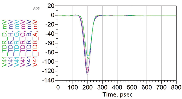
Figure 2. Circuit and simulated far-end noise.
The far-end crosstalk scales linearly with the coupled length and inversely with the rise time. We define the far-end crosstalk coefficient to take into account these scaling terms as:
 (3)
(3)
The effective dielectric constant is extracted for each line or differential pair from the time delay and the length using
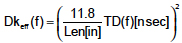 (4)
(4)
The time delay of each line or pair is calculated from the phase of the insertion loss in the frequency domain. The phase is unwrapped into the total delay, in cycles, and then scaled with the frequency,
 (5)
(5)
The delay, and effective Dk, is calculated for the single-ended lines and the odd and even mode cases.
Results and Interpretation
The most severe test of the field solvers is in the case of tightly coupled lines, and the results are reported here.
Impedance. The even and odd mode impedances are affected by coupling. The even mode impedance will be higher than the single-ended impedance, and the odd mode impedance will be lower than the single-ended impedance.
FIGURE 3 shows the relative values of the single-ended odd mode and even mode impedances for the six different tools.


Figure 3. Impedance variation for (top) microstrip structure and (bottom) stripline structure.
From Figure 3 (top), the value of Z0 for microstrip differential pairs shows a variation of ±0.6% for all the tools but D. Similarly, values of ZODD and ZEVEN show a variation of ±0.7% and ±0.7%, respectively. Tool D is not a field solver, but uses an approximation. It shows a higher value of impedance for Z0, ZODD and ZEVEN.
From Figure 3 (bottom), the value of Z0 for stripline differential pairs shows a variation of ±0.8% for all the tools but D. Similarly, values of ZODD and ZEVEN show a variation of ±1.3% and ±1%, respectively. These results simply state the variation in the predicted Z0, ZODD and ZEVEN is within 1% of each other for all the tools when used for the same geometry and with the same simulation parameters. This is the expectation of most users.
Dielectric constant. For a microstrip differential pair, the differential signal will have more field lines in air than the common signal. This will give the differential signal a lower effective dielectric constant and a higher speed, which essentially means the differential signal will have lower time delay than the common signal. This shows up in FIGURE 4, which compares the variation of DkSE, DkDifferential and DkCommon.


Figure 4. Dielectric constant variation for (top) microstrip structure and (bottom) stripline structure.
From Figure 4 (top), we see that, independent of tool D, which is not a field solver, DkSE shows a variation in values of ±1.2%. DkDifferential and DkCommon show a variation of ±1.2% and ±0.95%, respectively, for microstrip differential pairs.
For stripline differential pairs, we would expect no difference in the dielectric constant with the propagation mode, since the dielectric is assumed to be uniform and homogenous, independent of the field distribution.
The results in Figure 4 show a variation in DkSE values of ±0.5%. DkDifferential and DkCommon show a variation of ±0.5% and ±0.5%, respectively.
The agreement for dielectric constant is within 1% for both microstrip and stripline, for each of the field solver-based tools.
Near-end crosstalk (kb). The near- and far-end crosstalk features are very sensitive measures of the accuracy of a field solver, since these effects are fringe field dominated.
Given the tight coupling between the two lines in each pair, we would expect the near-end crosstalk to be large, on the order of 10%.
The simulated near-end crosstalk coefficients, extracted from a time domain simulation of the 4-port S-parameters, show values for both microstrip and stripline of about 10%, and all agree with each other to about within ±0.5%. These are shown in FIGURE 5.
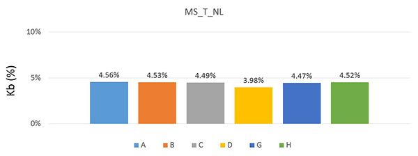

Figure 5. kb variation for (top) microstrip structure and (bottom) stripline structure.
Far-end crosstalk (kf). Far-end crosstalk is the noise on the quiet line, which propagates in the direction of the signal on the aggressor line. Far-end crosstalk scales with coupled length and inversely with rise time. This makes it frequency-dependent.
Instead of plotting the far-end coupling in the frequency domain terms, we calculated the coupling coefficient as described above.
From Equation 3 we can see k-coefficient is directly proportional to the voltage induced on the victim line. A higher value of k-coefficient corresponds to a higher level of far-end crosstalk. FIGURE 6 shows the variation of k-coefficient, and a close look tells us this variation is not much among the tools, which justifies that all the tools behave in a similar fashion. The variation in k-coefficient for microstrip line is ±0.9% for all the tools but D, which is an approximation. As expected, all the tools predict no far-end crosstalk in stripline.

Figure 6. kf variation for microstrip structure.
Conclusion
Our aim was to extract four important figures-of-merit and look at their variation for different tools, using microstrip and stripline differential pairs. Looking at the plots for different parameters and calculating the percentage variation among the tools for each of them, it is clear all the tools evaluated in this study offer results within about 1% of each other. While this is expected as an end-user, it is still remarkable, considering the tools use different approaches and different code to calculate S-parameters.
Acknowledgments
We would like to thank Nanya Technologies for its support in partially funding this project. We would also like to thank Dr. Don DeGroot from CCN Labs and Dr. Melinda J. Piket-May from CU Boulder for their valuable insights and discussions throughout the course of this project.
References
Eric Bogatin, Signal and Power Integrity – Simplified, second ed., Boston, MA: Prentice Hall, 2004.
P. G. Huray, The Foundations of Signal Integrity, Wiley-IEEE Press, 2009.
Eric Bogatin, Don DeGroot, Paul G. Huray, Yuriy Shlepnev, “Which One is Better? Comparing Options to Describe Frequency Dependent Losses,” DesignCon, January 2013.
V. Stajonanovic, M. Horowitz, “Modeling and Analysis of High-Speed Links,” Custom Integrated Circuits Conference, September 2003.
Dr. Alan Blankman, App note: “Characterizing Crosstalk with Aggressor On/Off Analysis Using SDAIII - CompleteLinQ,” Teledyne LeCroy, January 2013.
C. Warwick and F. Rao, App note: “S-parameters Without Tears,” Agilent Technologies, January 2010.
P. Triverio, “Stability, Causality, and Passivity in Electrical Interconnect Models,” IEEE Transactions on Advanced Packaging, November 2007.
Y. Shelpnev, “Quality of S-parameters Models,” Asian IBIS Summit, Nov. 18, 2011.
S. Hall and H. Heck, Advanced Signal Integrity for High-Speed Digital Designs, Wiley-IEEE Press, 2009.
Simbeor THz Electromagnetics Signal Integrity Software.
Advanced Design System (ADS) Electronic Design Automation Software.
Mentor Graphics HyperLynx – PCB Analysis and Verification Tool.
Sonnet Software Sonnet Suites 15.54.
Polar Instruments Si9000e PCB Field Solver.
Quite Universal Circuit Simulator QUCS Project.
Gaurav Narula will be receiving his master’s in electrical engineering in May 2016 from the University of Colorado Boulder. Dr. Eric Bogatin is adjunct professor, Dept. of ECEE, University of Colorado, Boulder and is dean of the Teledyne LeCroy Signal Integrity Academy(bethesignal.com); This email address is being protected from spambots. You need JavaScript enabled to view it..