Datasheet Df values are adequate, but copper roughness is critical. 

Virtually any PCB design today will have high-speed signaling, and accurate impedance and insertion loss modeling will be critical for the success of the design. Impedance modeling has evolved into a standard exercise, and most designers and fabricators have enough experience with it to be confident that their modeled and measured impedances will be very similar. Insertion loss modeling, on the other hand, is a relatively new requirement and very few people know exactly which parameters are most important for correlation between measurement and modeling. For instance, can I trust the 1GHz Er and Df values, or do I need the 10GHz values? While at Intel, I led an effort to determine the critical parameters. In our experience, the material property values commonly given on datasheets were adequate, but accurate copper roughness modeling was a key factor for proper correlation.

A study was performed to attempt to correlate measured insertion loss to that modeled with an Intel-proprietary 2D modeler (“QRLGC”), as well as a commercially available tool (Polar Instruments' Si9000e). We assembled a collection of coupons representing a broad range of materials and vendors, US and Chinese. The insertion loss of several coupons of each sample was measured using SET2DIL (without significant variation between coupons), and then the coupons were cross-sectioned to obtain the actual trace dimensions for each design. We also had access to the design files for each coupon, giving us the material used and design dimensions.

FIGURE 1 shows the final 4GHz correlation between measurements (blue), Intel’s “QRLGC” tool (red), and Polar’s Si9000e (green). Note that for most cases the correlation is within 5%, with samples 2 and 12 being the exceptions (variances of 12% and 8%, respectively). A large range of materials and subsequent loss values are represented, indicating insertion loss modeling is valid for a broad range of material properties and copper roughness. Later we also found IT-158 (such as used in sample 2) sometimes measured higher than expected loss in some other designs, depending on the manufacturer. We suspect something in the manufacture of laminates using this material occasionally
causes higher than expected losses. In case 12 (Meg-6), the Polar model correlated better than the Intel tool, perhaps because of a more representative copper roughness model.

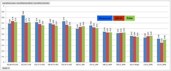
FIGURE 1. Final measurement vs. model correlation.

The initial correlation was not as impressive, and we learned quite a bit about what needs to be accurate for good correlation, and what has little or no effect. The first thing we found was that the 1GHz Dk (dielectric constant, or “Er”) and Df (dissipation factor, or loss tangent) values in the material datasheets could be used “as is” for good correlation at 4GHz and 8GHz. The slope of the insertion loss curves showed this. The modeling tools have built-in compensation to adjust those values for higher frequencies (Er and Df must vary with frequency, although only slightly for low loss materials above 1GHz), and those seem to work well.

We usually did not see a significant difference between tools, except for the samples with the roughest copper. As Figure 1 shows, there was usually only a small difference between the Intel and Polar modeling tools. It’s interesting to focus on samples 3, 4 and 5, which had the roughest copper. Note that the Polar tool, which uses the Hammerstad copper roughness model, consistently estimated less insertion loss for the roughest coppers than the Intel tool, which uses the Huray model for rough copper. This is to be expected; a modified Hammerstad model is appropriate for the roughest coppers.1 I suspect most tools will correlate well to each other, except for how copper roughness is handled.

Proper copper roughness compensation was the major variable that needed to be adjusted properly for good correlation. Intel had experience with various levels of roughness and its impact on insertion loss, and had on-hand values to use for Huray models for the copper roughness typically found on standard, RTF, VLP and HVLP coppers. Similarly, Polar modeled copper roughness based on cross-section measurements. Without proper copper roughness representation, correlation was much worse; this was the critical parameter to “get right.” These values still appear to have room for improvement, since the samples with the roughest copper (samples 3, 4 and 5) consistently underestimated loss.

Trace Resistivity

Another key aspect for proper correlation was the actual resistivity of the traces. Rather than being pure copper, manufactured PCB traces seem to have enough impurities in the “copper” to bring its conductivity down from ~5.9e7 S/m for pure copper to ~4.7e7 S/m for PCB traces. This value should be used for proper modeling of PCB “copper.”

A variable that didn’t prove significant in this study was the difference between using the actual measured geometries and those specified in the design. We had a standard rule that prevented manufacturers from varying any trace width or dielectric thickness by more than 0.5 mils from that specified, and it appears to have limited the variation in dimensions adequately to properly predict insertion loss.

Most of our correlation work was done at 4GHz, but we also checked the results at 8GHz, and the correlation was off by approximately twice the 4GHz value, indicating the percentage error was consistent across that frequency range.

This study proved reassuring in that no extreme measures were needed to get good correlation between measurements and models at 4 and 8GHz. The 1GHz Dk and Df values commonly available proved accurate for these frequencies. Copper roughness, especially on the roughest samples, proved the most challenging aspect to get correct. The modeling tools need to have settings for roughness dimensions, which are commonly available from cross-sectioning, and those dimensions must be obtained after all processing is complete; oxide alternative treatments can roughen the raw copper substantially. Of course, as frequencies get higher, further refinement will probably be necessary. For instance, on symmetric stripline, the roughness of both the top and bottom of the traces will be equally important, and they may have significantly different roughness profiles. Unique settings for each surface will be necessary. PCD&F

References

1. Yuriy Shlepnev and Chudy Nwachukwu, “Roughness Characterization for Interconnect Analysis,” 2011 IEEE International Symposium on Electromagnetic Compatibility (EMC), August 2011.

Jeff Loyer is signal and power integrity product manager at Altium (altium.com); This email address is being protected from spambots. You need JavaScript enabled to view it.. He spent more than 20 years as an engineer at Intel, the past 10 as signal integrity lead.