When optimizing board area when considering thermal effects, the IPC charts aren’t enough.
Prior to 2009 board designers concerned about PCB trace temperatures really had only one tool available to them. That tool started out as a poorly controlled, “tentative” set of curves created by two employees of the National Bureau of Standards in 1956 (Note 1). Those curves were redrawn and republished until they finally appeared in a military standard1 and ultimately in an IPC standard2. Board designers have been using them (and various calculators and Web pages based on them) ever since.
Finally, in 2009 IPC published a new standard, IPC-2152, Standard for Determining Current Carrying Capacity in Printed Board Design.3 This is arguably the first, best-researched, well-controlled, most complete investigation into trace current and temperatures in the history of our industry. It is over 90 pages long and contains over 75 charts and tables. There are only two problems with the standard: it is bulky and awkward to use, and the problem of trace currents and
temperatures is too complicated to be able to distill into a collection of charts.
In this article we cover the basic background information needed to understand why traces heat up with current, convert the chart data into sets of equations, evaluate the charts and the equations using a thermal simulation model, and look at the sensitivity of the trace and formula results to other factors (such as adjacent traces and planes, different materials, etc.) (Note 2). The overriding conclusion of this article is that optimizing board area when considering thermal effects does not seem to be possible without the use of sophisticated thermal simulation software.
Background
The standard formula for the resistance of a copper trace or conductor is
R = (ρ/A) * L [Eq. 1]
where R = resistance in Ohms
ρ = resistivity of copper (typ. 1.7 µOhm*cm = 0.67 µOhm*in)
A = cross-sectional area of the trace or conductor
L = length of the trace or conductor
The resistivity of copper (indeed for most materials) is very sensitive to temperature, so its value is usually offered at a specific reference temperature, often 20˚C. The sensitivity of the resistivity of copper to a change in temperature is called the “thermal coefficient of resistivity” and is often given as 0.0039 per degree C. So the resistance of a copper conductor at any temperature different from the reference is found from Eq. 2,
R = Rref(1+ α*ΔT) [Eq. 2]
where Rref = resistance at the reference temperature (often 20˚)
α = thermal coefficient of
resistivity (0.0039/˚C), and
ΔT = the change in temperature
from the reference
temperature.
From Eq. 2 we can derive Eq. 3:
ΔT = ((R/Rref)-1) / α [Eq. 3]
Eq. 3 is the form whereby we can calculate the temperature change of a conductor if we know the resistance of the conductor at the ambient temperature and at some elevated temperature.
When we pass a current (I) through a trace on a PCB, there is power dissipated in the trace given by the relationship I2R. This power dissipation heats the trace. At the same time, the trace cools by conduction into the board material, convection into the air surrounding the trace, and by radiation away from the trace. A stable temperature is reached when the I2R heating effect just equals the cooling effect. So we can speculate that the temperature change follows the relationship shown in Eq. 4, where w = width of the trace and Th = trace thickness (so w+Th is proportional to the surface area).
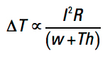 [Eq. 4]
IPC Curves and Equations
A typical IPC curve from IPC-2152 is shown in FIGURE 1. It has cross-sectional area (in square mils) along the horizontal axis and current along the vertical axis. Then individual curves are provided for various changes in temperature.

Figure 1. Typical IPC curve. Source: IPC-2152 Figure 5-1, p. 5.
We preferred working with curves which had current along the horizontal axis and the change in temperature on the vertical axis. This is more consistent with Eq. 4. So we converted a variety of curves in IPC-2152 to this orientation. We did that with the aid of a digitizing program (Note 3). We then fit equations to the resulting curves. A typical result for 2 oz. curves is shown in FIGURE 2.
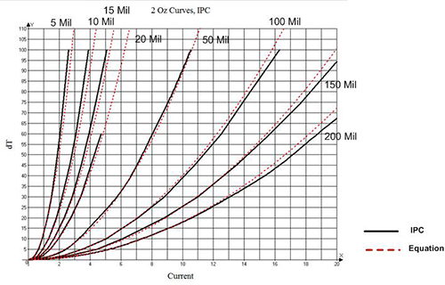
Figure 2. Converted 2 oz. IPC external data fitted with Eq. 4.
The IPC data are shown as the black curves in the figure, and our fitted equation (Eq. 5) is shown in each of the dotted red curves. Although not shown in this article, the curves and Eq. 5 matched equally well for all external trace sizes and currents. We believe an equation like Eq. 5 is much easier to deal with than are a large set of curves.
ΔT = 215.3 * C2 * W-1.15 * Th-1.0 [Eq. 5]
where ΔT = the change in temperature
from 20˚C
C = current in Amperes
W = trace width in mils
Th = trace thickness in mils (Note 4)
IPC-2152 also provides data for internal traces and traces in a vacuum. Perhaps the most surprising result in the standard is that internal traces actually run cooler than do external traces! This is a major change from the previous standard. The traces run cooler because the dielectric materials conduct heat away from the trace better than does the air.
Following the procedure above, we converted the internal and vacuum data to the format shown in Figure 2 and developed equations for those curves. The resulting equations are summarized in Appendix 1. The resulting equations are not as straightforward as Eq. 5, having different coefficients for some different trace widths. This can pose a problem when trying to design high-current traces on internal layers or in a vacuum, but the equations can, in fact, be pretty easily handled by calculators with appropriate programming (Note 5). In the cases where the formulas are different within a trace thickness, the differences are small and probably reflect errors, uncertainties and variations as a result of various graphical drawings and manipulations.
Thermal Simulations
We used a computer thermal simulation software tool (Note 6) to validate the IPC curves by modeling the IPC test board used for collecting the IPC data. The configuration of the test board used for the IPC testing is freely downloadable from IPC (Note 7). FIGURE 3 shows one of the images produced by the simulation and provides a good illustration of what the test board looks like. This particular simulation was of a 2 oz., 200 mils wide trace with 12A of current applied. The entire trace is 12" long with “sense” probes 3" in from each side. Insetting the probes from the trace edge helps minimize the effects of thermal gradients that might be caused by the presence of the pads. The resistance is measured between these probes with zero current (20˚C) and then with the test current (Note 8). The change in temperature is derived by applying Eq. 3.
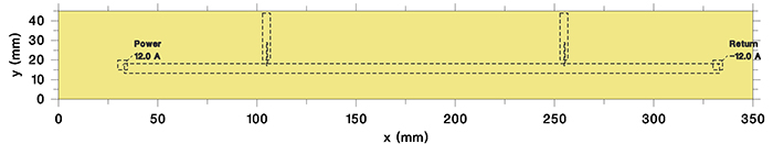
Figure 3. TRM model of a 2 oz., 200 mils wide trace.
FIGURE 4 shows the result of this simulation. The maximum temperature at the midpoint of the trace is 44.9˚C, which is a 24.9˚C change from the ambient. Note there are very definite thermal gradients away from the midpoint of the trace.

Figure 4. Result of simulation of the model shown in Figure 3.
Thermal simulations were run for a variety of 2 oz. external trace sizes and currents. Results of these simulations are plotted in FIGURE 5. The simulation results are the red squares on the diagram. The simulations fit the IPC derived curves and the equations very well. This high degree of congruence gives us a high degree of confidence in the IPC data, the equations and the simulations.

Figure 5. Thermal simulation results for selected curves.
Similar simulations were run for internal traces and traces in a vacuum. All simulations fit the IPC data and their derived equations quite well.
Sensitivities and Sensitivity Simulations
Be careful about certain sensitivities. One is how sensitive the change in temperature is to a change in current for very narrow traces. FIGURE 6 illustrates a close-up view of 1 oz. 5 mil and 10 mil wide traces. Note how the 5 mil wide trace change in temperature ranges from about 6˚ at a 500 mA current to about 25˚ at a 1.0A current to about 55˚ at 1.5A and 100˚ at 2.0A. A relatively small change in current can cause a really large change in temperature. The situation is slightly better for thicker traces.

Figure 6. Narrow curves are very sensitive to changes in current.
We ran several thermal simulations to examine the sensitivity of trace heating to a variety of factors. The control simulation was a 6" long, 1.0 oz., 200 mil wide trace carrying 15A, with pads at each end. A schematic of the model (similar to that shown in Figure 3) is shown in FIGURE 7. In this control situation, the change in temperature was 94.9˚, as shown in FIGURE 8.
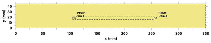
Figure 7. Schematic of thermal simulation of 6˚, 1 oz., 200 mil wide trace.

Figure 8. Thermal profile of the simulation in Figure 7.
One thing to notice from this simulation is the thermal profile. The hottest portion of the trace is at the midpoint (about 114.9˚C, which is 94.9˚ above ambient), as one would expect. But the temperature near the pads is much cooler, in this case about 60˚ above ambient. So when we are thinking about the maximum temperature of a trace, it is important to consider where that maximum temperature is going to occur.
If we do nothing but change the length of the trace, the results change:

The difference is likely caused by the impact of the pads. In this simulation, the pads were not connected to a power plane. If they were connected to a power plane, the plane would act as a heat sink, likely cooling the trace even more. Thus, changing the trace length can impact the change in temperature.
It takes time for a trace to reach a stabilized temperature. The time can be impacted by several things. But on the other hand, the simulations we looked at were reasonably uniform in this respect. FIGURE 9 illustrates the transient response for our control simulation. Although the temperature will continue to rise for a very long time (up to 30 min.), it has reached very close to its maximum temperature within about 5 min. This may or may not have implications for board designs.
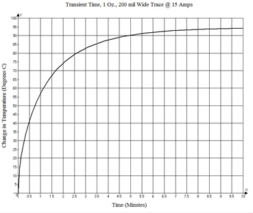
Figure 9. Transient response for 1 oz., 6”, 200 mil wide trace with a switched current of 15A.
An underlying plane has a major effect on the change in temperature. We simulated the case of a plane on the opposite side of a 63 mil thick board, and also a plane layer 10 mils under the trace. In both cases we modeled a continuous plane across the entire board. But all that is really needed is a plane that extends several trace widths in both directions from the trace. Without a plane, the change in temperature was 94.9°. With a plane on the opposite side of the board, the change in temperature was only 47.9°. But with a plane 10 mils directly underneath the trace (typical of many modern boards today), the change in temperature was only 33.7°C.
Figures 10 and 11 show the thermal gradients in the dielectric layer directly under the trace layer for the simulations with no plane and with a plane 10 mils under the trace. The dielectric is much hotter for the simulation without the plane. But the impact that the plane has in spreading the heat away from the trace is clear in Figure 11.
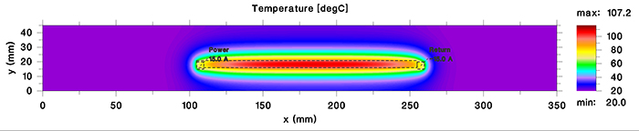
Figure 10. Thermal gradient in dielectric with no plane.
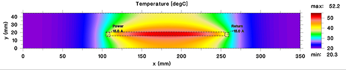
Figure 11. Thermal gradient in dielectric with a closely spaced plane.
We ran a simulation of our control trace next to a second, 200 mil wide trace placed 8 mils away (edge-to-edge.) The adjacent trace carried no current. The control trace cooled a little to a temperature change of 84.9˚. But the adjacent trace warmed to a temperature change of 51.5˚. This may or may not be an issue in board designs.
Finally, we looked at a different material. All IPC trace data are taken with traces on a board with polyimide dielectric. Polyimide has a slightly higher thermal conductivity than does FR-4, for example. Thus, polyimide will result in a slightly cooler trace than will standard FR-4. All our simulations above were done with the dielectric assumed to be polyimide. When the control simulation was run with FR-4 instead, the trace heated to a temperature change of 122.9˚ (instead of 94.9˚).
Board material is a very difficult parameter to analyze. The material properties will vary between manufacturers. Thermal conductivity will vary depending on the direction; that is, the thermal properties in the X-Y direction will be different from the thermal properties in the Z direction. Materials with “tighter” weave will probably cool better than will materials with “looser” weaves. There are no dependable standards for measuring and reporting thermal conductivity. Therefore, board thermal characteristics may change somewhat if the material is changed (either knowingly or unknowingly).
After looking at several different simulations based on our control simulation of a 1 oz. 200 mil wide, 6" long trace carrying 15A and a polyimide board material, the results are a little less than comforting! They are summarized in TABLE 1.
Table 1. Results of Control Simulation

Conclusions
As a result of the simulations, we can offer a couple of conclusions:
- It is almost universally true that variations in results increase with temperature. That is, at low temperatures (associated with lower currents) the various parameters we have looked at here make little or no difference. At intermediate temperatures, the differences would by much milder than reported here.
- Except for material selection, the IPC curves generally represent a “worst case” scenario. Any other variation we introduce lowers the trace temperature, sometimes considerably so.
- We have not addressed in this paper some of the more complex shapes such as fillets in thermal reliefs or copper plating in drill holes. While we can speculate that the I2R heating in these cases might be similar to other simulations, the cooling situations might be substantially more complicated.
One overriding conclusion is inescapable. The relationship between trace currents and temperatures is very complex. It is too complex to model with a single set of equations or curves. Since board real estate is very expensive, board designers usually want to use the smallest traces their fabricators will permit while still meeting requirements. Optimizing board area when considering thermal effects does not seem to be possible without the use of sophisticated thermal simulation software.
References
1. MIL-STD-275E, Printed Wiring For Electronic Equipment, Dec. 31, 1984.
2. IPC-2221, Generic Standard on Printed Board Design, February 1998.
3. IPC-2152, Standard for Determining Current Carrying Capacity in Printed Board Design, August 2009.
4. Douglas Brooks and Johannes Adam, “Trace Currents and Temperatures Revisited,” 2015, available at www.ultracad.com.
Notes
1. Ref. 3 contains a good historical summary of the development of the original charts. Ref. 4 contains copies of some of these early references.
2. This paper summarizes the results of a much more detailed paper by the authors4. Many of the details regarding curve fitting and thermal simulations are covered in much more detail in that paper.
3. We used a program called GetData Graph Digitizer, available at www.getdata-graph-digitizer.com.
4. This equation has thickness in mils, while all the curves show thickness in ounces. We used the following conversions: 0.5 oz. = 0.65 mils; 1.0 oz. = 1.35 mils; 2.0 oz. = 2.7 mils; 3.0 oz. = 3.9 mils.
5. UltraCAD’s PCB4.0 Trace Calculator handles these calculations easily.
6. The software tool we use is called TRM (Thermal Risk Management) developed by Dr. Johannes Adam. See adam-research.com for more information regarding the tool and these types of simulations.
7. IPC-TM-650, Test Methods Manual, method 2.5.4.1A “Conductor Temperature Rise Due to Current Changes in Conductors” available at www.ipc.org/test-methods.aspx.
8. The temperature change can be determined by measuring the change in resistance and applying Eq. 3, or measuring the change in voltage, dividing by the current (to get the change in resistance), and then applying Eq. 3. In either case, the change in temperature that is measured is the average change over the entire trace length, not the peak temperature change at the midpoint of the trace.
Douglas Brooks, Ph.D., is owner of UltraCAD Design, a PCB design service bureau and author of PCB Currents: How They Flow, How They React; This email address is being protected from spambots. You need JavaScript enabled to view it.. He will speak at PCB West in September in Santa Clara, CA. Johannes Adam, Ph.D., CID, is founder of ADAM Research, a technical consultant for electronics companies and a software developer, and the author of the Thermal Risk Management simulation program.