The state of reliability of the today’s complex and costly electronics and photonics systems should be checked (monitored) and, if possible and feasible, even managed on a continuous basis. This is particularly true for systems where failure-free operation is especially important. The objective of technical diagnostics (TD)1,2 is to recognize, in a continuous fashion and without taking apart the object of interest, its technical state and its ability to continue to perform in the expected (specified) fashion. TD establishes the links between the observed (detected) signals, the so-called “symptoms of faults” (SoF), and the underlying hidden state (“health”) of the device or the system of interest. TD effort is naturally focused on the most vulnerable elements (weakest links) of the design and can use the failure-oriented accelerated test (FOAT) data3 conducted in the design stage.
TD is an important part of reliability engineering and encompasses a broad spectrum of problems associated with obtaining, processing and assessment of diagnostic information, including diagnostic models, decision making rules and algorithms. TD provides information for the subsequent prognostics and health monitoring/management (PHM) effort.4 TD has to devise solutions and recommendations (“educated guesses”) under conditions of uncertainty and with limited information. Therefore the TD methods, techniques and algorithms are based, as a rule, on the probabilistic risk management and applied probability bodies of knowledge and are supposed to quantify, on the probabilistic basis, the obtained information (signals, SoF) and to provide assistance in making a decision if the device or a system of interest is still sound or has become faulty. There is always the possibility that the interpretation of the obtained SoF signal might be a false alarm or might lead to a missing-a-target decision. Statistical theory of decision-making, which is widely employed in radar engineering and is part of the TD, can be effectively used to avoid a false-alarm/missing-a-target mistake.
The objective of the analysis that follows is to show how the statistical Bayes formula (theorem) to update beliefs5-10 can be used to interpret the TD (PoF) information and to determine if the device (system) of interest is still sound (healthy) or has become faulty, and to use this information to identify a faulty device, if any. Then a reliability physics-oriented Boltzmann-Arrhenius-Zhurkov (BAZ) model11-13 can be employed to estimate the remaining useful lifetime (RUL)4,14 of a damaged (faulty) device. When the PDfR concept is used,2,15 such an assessment will lead, of course, to different RUL predictions, depending on the level of the allowable probability of failure (PoF).
Bayes formula in TD problems. Bayes’ theorem to update beliefs is widely used in many areas of applied science, engineering, economics, game theory, medicine and even law. In this section we interpret the Bayes’ formula in application to TD problems.
Let an event S be the observed (detected) signal (SoF), such as, e.g., measured elevated off-normal temperature, elevated leakage current, drop in the output light intensity, elevated amplitudes (power spectrum) of the induced vibrations, etc., and the events Di, i = 1,2,3...be possible malfunctions, diagnosed deviations from the normal operation conditions of the product (system) elements that might be responsible for the observed symptom(s). It is assumed that one and only one of the product elements is damaged to an extent that its detected off-normal performance has manifested itself in the observed symptom. Simultaneous failure (damage) of two or more systems’ elements is deemed to be extremely unlikely and is excluded from consideration.
Let one know the typical probabilities P(Di) of failure of its particular elements, based on the accumulated experience for the type of the device or system in question. The problem of interest can be formulated this way: The event (signal) S is observed for the given device (system) in operation. What is the probability that it is the system’s particular i-th element that has become faulty and is therefore responsible for the detected symptom?
The Bayes formula
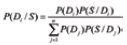
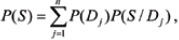
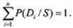
enables one to determine the posteriori probability P(Di)/S), after the symptom S has been detected, from the priori probability P(Di) of the typical, known from the previous experience, probability of the system’s state. The Bayes formula can be obtained from the complete probability formula
and the relationship
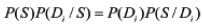
Formula 2 reflects a postulate that if a system has several possible and incompatible ways to get transferred from the state Dj to the state S, the probability of such an event can be found as the sum of the conditional probabilities of occurrence of each of these ways. Formula 3 indicates the probability of the simultaneous occurrence of the symptom S and the system condition (diagnosis) Di.
As follows from Bayes formula,
Bayes method is simple, easy-to-use and effective, and is widely used in many applied problems. Its shortcomings are the large volume of the required input information and “suppression” of seldom diagnoses.
Example 1. Let it be established from experience with the given devices or systems that 90% of the devices do not fail during the designated time of operation, and the symptom S, which is the increase in temperature by 20˚C above the normal level, is encountered in 5% of the cases (devices). The probabilities P(D1) and P(D2) of the sound condition D1 and the faulty condition D2, respectively, in the general population of devices are P(D1) = 0.9 and P(D2) = 0.1, respectively. The conditional probabilities are P(S / D1) = 0.05 and P(S / D2) = 0.95. Let us determine the probability that the device, in which the increase in temperature is detected, is sound. The Bayes formula yields

Thus, the probability that the device is still sound has decreased because of the detected increase in the observed temperature, from 0.90 to 0.32.
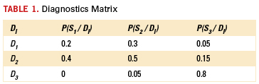
Example 2. The TD instrumentation has detected two deviations (SoF) from normal operation conditions: increase in temperature by 20˚C in the region of the heat sink location (symptom S1) and increase in the power of the vibration spectrum by 20% (symptom S2). It has been established that these symptoms might be due to the possible malfunction of one of the two pieces of hardware: heat sink (state D1) and/or vibration damping equipment (state D2). It has been established also that the symptom S1 (increase in temperature) is not observed at normal operation condition (state D3), and the symptom S2 is observed in 5% of cases (devices). Based on the existing experience of employing the devices of interest, it has been established that 80% of the devices do not fail during the specified time of operation; 5% of the devices are characterized by the state D1 (malfunction of the heat sink), and 15% are characterized by the state D2 (malfunction of the vibration damping system). It also has been established that the symptom S1 is encountered in the state D1 in 20% of the devices, and in the state D2 in 40% of the devices; that the symptom D2 is encountered in the state D1 in 30% of the devices, and in the state D2 in 50% of the devices. This information can be conveniently presented in the form of a diagnostic matrix (Table 1).
Let us determine first the probabilities of the device states, when both symptoms, S1 and S2, have been detected. The Bayes formula1 yields

Similarly, we find: P(D2 /S1S2) = 0.91; P(D3/S1S2) = 0. Determine now the probability of the device state, if the observations indicated that there was no increase in temperature (the symptom S1 does not take place), but the symptom S2 (increase in the power spectrum of the induced vibrations) was detected. The absence of the symptom S1 means that the symptom  of the opposite event takes place, so that
 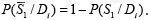 . Changing the probability P(S1/Di) in the diagnostics matrix to
  we find

Similarly, we obtain 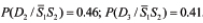 : Determine now the probabilities of the device states when none of the symptoms takes place. By analogy with the above calculations, we find

Similarly, we obtain: 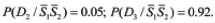 The calculations indicate that when both symptoms S1 and S2 are observed, the state D1 (the heat sink is malfunctioning) might occur with the probability 0.91. When none of these symptoms is observed, the normal state D3 is characterized by the probability 0.92 and is the most likely one to occur. When the symptom S1 (elevated temperature) is not observed, while the symptom S2 (elevated vibrations) is, the probabilities of the states D2 (damping system is not working properly) and D3 (both heat transfer and vibration damping hardware work normally) are 0.45 and 0.41, respectively. Since these probabilities are close, additional information based on observations and/or modeling might be needed to obtain more accurate diagnostics information.
Boltzmann-Arrhenius-Zhurkov’s (BAZ) model. Bayes formula (1) does not require any information about the physical nature of the obtained signals. When there is a reason to believe that the combination of elevated temperature and stress (not necessarily mechanical) can lead to a malfunction of a device or a system, the additional information about the possible source of the deviation of the system’s state from the normal operation conditions could be obtained by using Boltzmann-Arrhenius-Zhurkov (BAZ) model11-13
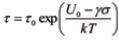
that enables one to evaluate the mean time to failure (MTTF) τ from the known applied stress σ (not necessarily mechanical); the absolute temperature Τ, the time constant τ0, the (stress-independent) binding (activation) energy U0; k = 1.3807 x 10⁻²³J/0K is Boltzmann’s constant, and the factor γ is the material (device) constant that is a measure of the vulnerability of the material to the applied stress and is measured by energy per unit stress, so that the product γσ measured in energy units.
BAZ model proceeds from the rationale that although the process of accumulation of damages is temperature dependent, it is influenced primarily by an external loading of any relevant nature. In other words, the model is based on the recognition of the experimentally observed situation that the breakage of the chemical bonds in a material under stress is due primarily to this stress, while temperature plays an important, but not a prevailing, role. Since the BAZ model contains three empirical parameters, activation energy U0, parameter γ of the level of the disorientation of the molecular structure of the material, and the time constant τ0, three failure-oriented accelerated test (FOAT) series should be conducted to determine these parameters.
Let FOATs characterized by their absolute temperatures T1, T2 and T3 and applied stresses σ1, σ2 and σ3 be run until failures, and the respective measured times-to-failure (TTF) be t1, t2 and t3, respectively. Based on the observed percentages of failed devices, the probabilities of failure (PoF) where established are Q1, Q2 and Q3 respectively. Assuming that the BAZ model and the exponential law of reliability are applicable, the PoF can be defined as
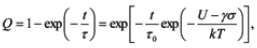
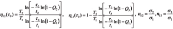
where t is time in operation. The time constant t0 in the BAZ model can be found from the transcendental equation
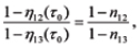
where the following notation is used:
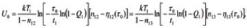
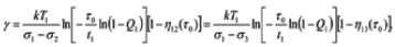
Then (stress-free) activation energy U0 and the factor γ of loading (power) in the BAZ model can be computed as
Example 3. Let, e.g., the FOAT carried out until half of the population fails
(Q1 = Q2 = Q3 = 0.5) indicate that
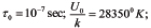
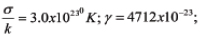
so that 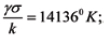 then, for the operation temperature of T = 110˚C = 383˚K, the BAZ formula yields:
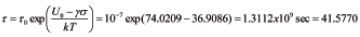
years. The MTTF will decrease to

years. For the 20˚C increase in temperature, and will be only

days for the 20% increase in the power of the vibration spectrum. Although, as is evident from the obtained data, the faulty damping hardware could result in a significantly lower lifetime than the defected heat removing hardware; the damage in the damping hardware, based on the Bayes formula prediction, is much less likely than that in the heat sink.
Example 4. Let us define the remaining useful lifetime (RUL) as the time between the moment when the diagnostic instrumentation has detected the malfunction (in the case in question it is the heat sink) and the moment of time when the PoF reached the allowable level Q. Assuming that the exponential law of reliability is valid (this law is characterized by the largest entropy and, hence, is the most conservative one), we find the RUL as
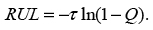
Assuming, e.g., Q = 10-3, we conclude that although the RUL is only  years = 2.4070 days,
this time is sufficient, however, to replace the faulty heat sink or the heat spreader or to fix the damage. If, however, the specified allowable level of the PoF is as low as Q = 10-5, the expected RUL becomes as short as
 years = 34.6min.
There is not very much that could be done to restore the system’s reliability and to maintain it on the high level.
Conclusion
By combining the statistical Bayes formula and the physical BAZ model, one can obtain useful diagnostic information about the state of an electronic or photonic device or a system, subjected to the temperature-vibration bias. This information can be used as input data for the subsequent PHM effort. The suggested methodology is viewed as part of the general PDfR approach and can be used in the analysis, design and operational reliability assurance of electronic and photonic devices and systems, when reliability is imperative and its quantification is therefore a must.
References
1. H. Czilos, ed., “Handbook of Technical Diagnostics,” Springer, 2013.
2. E. Suhir, “Applied Probability for Engineers and Scientists,” McGraw-Hill, 1997.
3. E.Suhir, R.Mahajan, “Are Current Qualification Practices Adequate?” CIRCUITS ASSEMBLY, April 2011.
4. M.G. Pecht, “Prognostics and Health Management of Electronics,” John Wiley, 2008.
5. S.B. McGrayne, “The Theory That Would Not Die: How Bayes’ Rule Cracked The Enigma Code, Hunted Down Russian Submarines, & Emerged Triumphant from Two Centuries of Controversy,” New Haven: Yale University Press, 2011.
6. T. Bayes and R. Price, “An Essay Towards Solving a Problem in the Doctrine of Chance.” By the late Rev. Mr. Bayes, communicated by Mr. Price, in a letter to John Canton, M. A. and F. R. S. Philosophical Transactions of the Royal Society of London, 53 (0), 1763.
7. L. Daston, “Classical Probability in the Enlightenment”. Princeton Univ Press, 1988.
8. S.M. Stigler, “Who Discovered Bayes’ Theorem?” The American Statistician 37(4), 1983.
9. Edwards, A. W. F. (1986), “Is the Reference in Hartley (1749) to Bayesian Inference?” The American Statistician, 40(2), 1986.
10. S.E. Fienberg, “When Did Bayesian Inference Become ‘Bayesian?’ ” Bayesian Anal., Jan. 2006.
11. S. N. Zhurkov, “Kinetic Concept of the Strength of Solids,” Int. J. of Fracture Mechanics, vol. 1, no. 4, 1965.
12. E.Suhir, R. Mahajan, A.E. Lucero and L. Bechou, “Probabilistic Design-for-Reliability Concept and Novel Approach to Qualification Testing of Aerospace Electronic Products,” IEEE Aerospace Conference, March 2012.
13. E. Suhir, “Predicted Reliability of Aerospace Electronics: Application of Two Advanced Probabilistic Concepts,” IEEE Aerospace Conference, March 2013, to be presented and published.
14. E. Suhir, “Remaining Useful Lifetime (RUL): Probabilistic Predictive Model,” International Journal of PHM, vol. 2(2), 2011.
15. E. Suhir, “Probabilistic Design for Reliability,” Chip Scale Review, vol. 14, no. 6, 2010.
Ephraim Suhir, Ph.D., is Distinguished Member of Technical Staff (retired), Bell Laboratories’ Physical Sciences and Engineering Research Division, and is a professor with the University of California, Santa Cruz, University of Maryland, and ERS Co.; This email address is being protected from spambots. You need JavaScript enabled to view it.. Laurent Bechou, Ph.D., is a professor at the University of Bordeaux IMS Laboratory, Reliability Group. Alain Bensoussan is EEE senior parts engineer, Thales Alenia Space France.