Although final performance is measured in the time domain, a detour may be the faster route to a signal integrity solution.
Do you speak frequency domain? Especially if you are a digital designer, you should consider learning the language of the frequency domain. The time domain has special significance because it is the real world. This is the domain in which we live our lives, where we build our intuition, and where we measure digital performance. If the time domain is the real world, why would we ever want to leave to enter the frequency domain?
For signal integrity problems related to lossy transmission lines, working in the frequency domain can often help us find solutions to eye closure problems.
Sometimes, taking a detour through the frequency domain can bring an acceptable answer more quickly than staying in the time domain.
In this brief introduction to solving problems in the frequency domain, we will look at how to improve signal quality in high-speed serial links like PCI Express (PCIe) by speaking the language of the frequency domain.
Rise time in the frequency domain. If the time domain is the real world, what does this make the frequency domain? The frequency domain is not the real world; it’s a mathematical construct. As such, it has certain very special rules that must be followed. One rule is that only sine waves can be used to describe signals.
Each sine wave is described by a frequency, an amplitude and a phase. While the phase of a sine wave is important, we usually focus attention on the amplitude of the sine wave.
Any waveform in the time domain can be translated into the frequency domain using the Fourier Transform. While it is important to have done a Fourier Transform by hand at least once in your life, after that, it’s usually more important to get the answer as quickly as possible. Every version of SPICE can perform a Fourier Transform of any arbitrary time domain waveform.
The hidden assumption with these translations, typically called a Discrete Fourier Transform, or DFT, is that the waveform in the time domain is repetitive. The repeat frequency is either the clock frequency or the total simulation time. The repeat frequency has special significance. It is the lowest frequency that will appear in the spectrum and is called the fundamental frequency.
Every frequency component that appears in the frequency domain is a multiple of this fundamental and is called a harmonic. The collection of all the harmonic components is called the spectrum.
A very important waveform in the time domain and the frequency domain, to which most other waveforms are compared, is an ideal square wave. In the time domain, an ideal square wave has a zero psec rise time and a 50% duty cycle.
Its spectrum has three important features:
- Only multiples of the fundamental appear.
- The harmonic of each component drops off like 1/n, the harmonic number.
- The even harmonics, i.e., 2d, 4th, 6th, etc., have zero amplitude.
For an ideal square wave, the frequency components continue with their pattern to infinite frequency, always dropping off inversely with frequency or harmonic number. But, if the rise time is finite, this is not the case. After some frequency, which we call the bandwidth, the amplitudes of the frequency components drop off much more quickly than 1/f for an ideal square wave.
Figure 1 shows a 1 GHz ideal clock square wave spectrum and the spectrum of a clock with a rise time that is 5% the clock period. The relationship between the 10-90 rise time, RT, and the bandwidth, BW, is roughly approximated as BW = 0.35/RT. For this example, we would expect the bandwidth to be about 0.35/0.05 = 7 GHz. This is about where the amplitude begins to drop off below the ideal square wave spectrum.
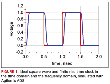
Every frequency component of an ideal square wave is significant in contributing to that 0 psec rise time. However small the amplitude may be at very high frequency, it is still important. Remove any and you won’t get the 0 psec rise time.
When the frequency component of a real waveform has an amplitude significantly smaller than the equivalent ideal square wave, it won’t be large enough to contribute to the rise time and can be ignored. The bandwidth of a real waveform is the highest sine wave frequency component that is significant. Decrease its bandwidth in the frequency and its rise time in the time domain will increase.
A fundamental measure of the rise time of a signal in the time domain is the frequency at which the harmonics begin to drop off more quickly than 1/f. For this reason, the bandwidth is often referred to as the knee frequency. The lower the knee frequency in the frequency-domain, the longer the rise time of the signal in the time-domain.
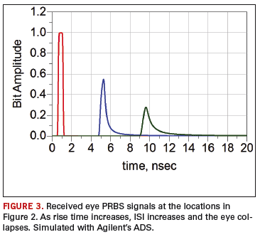
Signal propagation on real interconnects. How do real interconnects like traces on a circuit board, or coax or twin-ax cables, affect signals? In the time domain, we can evaluate the behavior of a single bit as it propagates down a transmission line. Figure 2 shows what a single 1 bit would look like traveling down a 0.003˝ wide FR-4 transmission line for a 1 Gbps signal, initially, after 30˝ and after 60˝.
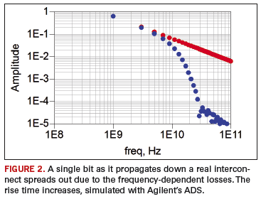
The single 1 bit starts out with a 1 nsec unit interval, and a very fast rise time. As it propagates down the transmission line, the wave form is dramatically affected. That single bit spreads out into adjoining bits. This cross talk between one bit and other bits is called inter-symbol interference or ISI. It contributes to the collapse of the eye. Figure 3 shows the received eye of a pseudo random bit stream (PRBS) signal at the three locations above.
How the single bit spreads out is a very important metric of the behavior of the interconnect. Yet, as viewed in the time domain, the exact shape of the pulse is complicated and difficult to describe in a simple way.
Here is where the frequency domain description offers a simpler description. The term that describes how a sine wave differential signal is affected by an interconnect when it exits is the differential insertion loss, sometimes referred to by its S-parameter designation, SDD21. This is also called the transfer function of the interconnect. This measureable property describes what a sine wave with amplitude of 1 looks like when it comes out the transmission line. The differential insertion loss for these interconnect paths is shown in Figure 4.
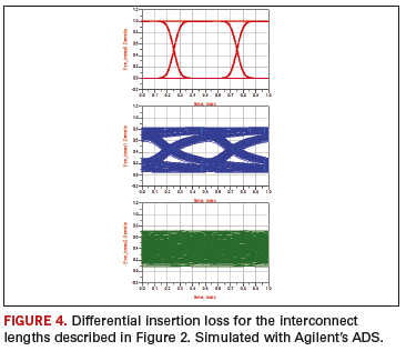
Every single interconnect has a similar SDD21 response. The amplitude coming out is always less than the amplitude going in, and the amplitude of SDD21 drops off with increasing frequency. On a log scale of amplitude, measured in dB, the differential insertion loss generally drops off nearly linearly with frequency. A metric of the dB/inch per GHz is one single number that characterizes most interconnects.
If we send an ideal square wave signal into a real interconnect, its spectrum will be multiplied by this transfer function. The SDD21 tells us how each frequency component will be attenuated. Higher frequencies get attenuated more than lower frequencies. This pushes the knee frequency of the signal’s spectrum to lower frequency, and increases the rise time of the signal.
This frequency-dependent attenuation of typical interconnects will cause rise time degradation, which will smear one bit into adjacent bits, result in ISI and cause collapse of the eye.
It’s not the attenuation of the interconnect that degrades the rise time; it is the frequency dependence of the attenuation. After all, if we take all the frequency components and just attenuate each of them the same amount, we will still have the same spectral shape of the bit sequence coming out. The frequency at which the knee occurs will be unchanged; the rise time of the signal will be unchanged, and there will be no ISI and no collapse of the eye.
Fixing the eye collapse in the frequency domain. We can fix the ISI in real interconnects by either flattening the insertion loss curve of the interconnect, or by changing the spectrum of the signal going into the interconnect so that when it comes out, it preserves the 1/f shape.
Designing an interconnect with a flatter response is tough. The root cause of the frequency-dependent loss is the combination of the skin depth dominated copper series resistance and the laminate material dielectric loss. For example, certain Gore cable assemblies use a very thin signal conductor, which has a frequency-dependent resistance much flatter than a typical copper core cable.
Likewise, laminates such as Rogers’ RO4350 have a lower dissipation factor and a flatter response dielectric loss curve. Both these interconnect design features reduce ISI with a flatter differential insertion loss response.
It is also possible to flatten an interconnect’s transfer function by adding some extra frequency-dependent gain at the receiver. If the interconnect has more attenuation at higher frequency, why not add gain that increases at higher frequency to compensate and flatten the overall response? Figure 5 shows how this works.
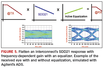
When we add frequency-dependent gain, we equalize the response of the interconnect across a wide frequency range. We call this process equalization. The ideal equalizer has a gain curve that is the exact inverse of the attenuation curve. With a flat response, the spectrum of the transmitter is preserved at the receiver; the knee frequency is the same as the transmitter; the rise time is the same, no additional ISI and no additional collapse of the eye.
Finally, the spectrum of the signal at the transmitter can be pre-distorted to add extra high-frequency components. The interconnect will attenuate the high-frequency components anyway. If we add extra high-frequency components at the transmitter, by the time they travel through the interconnect, they will be attenuated away, leaving the 1/f spectrum of a short rise time signal. The shorter the rise time, the less the ISI, and the lower the eye collapse.
One way of implementing adding high-frequency components is called pre-emphasis. Wherever a 1 bit begins, extra energy is added. Likewise, we could obtain the same pre-distorted spectrum by taking out low-frequency amplitudes. Whenever there is a string of more than one bit with the same value, reduce the signal level. This is called de-emphasis (Figure 6).
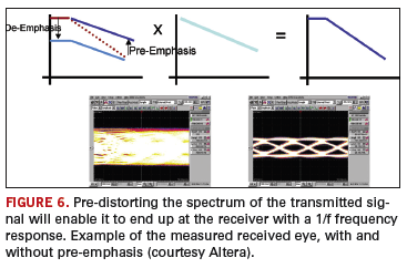
Both pre- and de-emphasis result in the same distorted shape in the transmitted signal spectrum. When either of these distorted signals travel through an interconnect, if optimized for the interconnect, the signal will come out the other end with a short rise time, less ISI and a more open eye.
By looking in the frequency domain, we can see how the techniques mentioned manipulate the frequency domain spectrum of the received signal. We engineer it to look more like an ideal square wave’s spectrum and recreate the shortest rise time to minimize its ISI and keep the eye open so that each bit can be detected as its true 0 or 1 value.
Even though final performance is always measured in the time domain, sometimes detouring through the frequency domain may be a faster route to a signal integrity solution.
Au: Many of the principles described in this paper are covered in great detail in papers that can be downloaded from bethesignal.com.
Eric Bogatin, Ph.D., is a signal integrity evangelist with Bogatin Enterprises (bethesignal.com); This email address is being protected from spambots. You need JavaScript enabled to view it..