 Data distribution, explained.
In my December column I listed three items to watch out for when evaluating capability study results: Cp versus Pp, the distribution of data, and sample size. I hopefully cast some light on the differences between the two measures of capability, Cp and Pp.
In this column I will dive deep into the distribution of data. The thing to remember is the standard capability study assumes the data are normally distributed. This assumption of normality, while not so critical in other statistical tools, is very important in capability studies.
Cp and Pp give us predictions based on a sample of how our population will behave in the far tails of the normal curve. These measures use mean and standard deviation to create a normal distribution, and, from this, predict how many of our parts, over the entire population of parts, will fall outside the tolerance limits.
If we assume our process is normally distributed, and measure Pp = 2.0 (Six-Sigma process), this means we are predicting extremely low ppm levels of defects: less than 0.002 ppm (3.4 ppm with the irritating 1.5 shift). What this means (regardless of your position on the 1.5 shift) is that if the data are not actually normal, we could either overestimate or underestimate our risk.
The figures demonstrate an example of this. Using Minitab, I generated 1,000 rows of random data using a Weibull distribution (shape = 1, scale = 100, threshold = 10). I somewhat arbitrarily chose 0 and 400 for spec limits. I performed a capability study using three variations: assuming the data were normal (FIGURE 1); assuming the data were Weibull (FIGURE 2); and assuming the data were normal but setting the zero lower limit as a lower boundary (FIGURE 3).

Figure 1. Weibull data calculated as normal. Ppk = 0.38, expected ppm outside limits = 127,006.
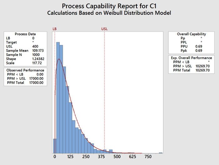
Figure 2. Weibull data calculated as Weibull. Ppk = 0.69, expected ppm outside limits = 102,069.
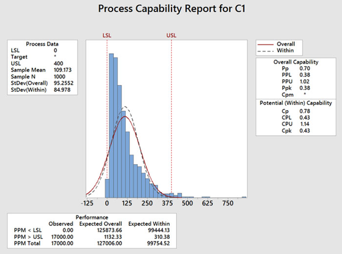
Figure 3. Weibull data calculated as normal. 0 = LB. Ppk = 1.02, expected ppm outside limits = 1132.
This example, while perhaps not the best, does illustrate several things. First, that one can get many different calculations for Ppk and “expected ppm defective,” depending on the assumptions. In this example, if the engineer did not check the distribution, but did realize that the lower spec limit was a lower boundary, they would assume the process had a Ppk of about 1.02. But if they checked the distribution and ran the study using a Weibull distribution, the Ppk would be worse – closer to 0.69.
The bottom line: be practical. I often attempt to find a distribution or transformation that fits, and if so, I use that to calculate Pp, etc.
But if I cannot find a good fit (for instance data that are heavily left leaning toward zero), we may find that the fit to normal is horrible, but the fit to other distributions is only marginally better.
I am not sure a professor of statistics would approve, but in these cases I do two things: One, I pick the distribution or transformation with the lowest Anderson-Darling value and run the capability study using that. I then create a time series plot (if the data are in time order) or a box plot and add the spec limits to that. This gives me a “practical” view of the range of the data in relation to the specification limits, and I can gauge whether my estimate of Ppk makes sense.
John Borneman is a Six Sigma Master Black Belt with over 40 years’ experience in electronics manufacturing; This email address is being protected from spambots. You need JavaScript enabled to view it..