The cost of improving and maintaining reliability can be minimized by a model that quantifies the relationships between product cost-effectiveness and availability.
A repairable component (equipment, subsystem) is characterized by its availability, i.e., the ability of the item to perform its required function at or over a stated period of time. Availability can be defined also as the probability that the item (piece of equipment, system) is available to the user, when needed. A large and a complex system or a complicated piece of equipment that is supposed to be available to users for a long period of time (e.g., a switching system or a highly complex communication/transmission system, whose “end-to-end reliability,” including the performance of the software, is important), is characterized by an “operational availability.” This is defined as the probability that the system is available today and will be available to the user in the foreseeable future for the given period of time (see, e.g., Suhir1). High availability can be assured by the most effective combination of the adequate dependability (probability of non-failure) and repairability (probability that a failure, if any, is swiftly and effectively removed). Availability of a consumer product determines, to a great extent, customer satisfaction.
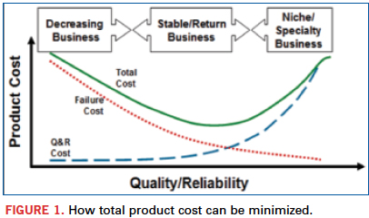
Intuitively, it is clear that the total reliability cost, defined as the sum of the cost for improving reliability and the cost of removing failures (repair), can be minimized, having in mind that the first cost category increases and the second cost category decreases with an increase in the reliability level (Figure 1)2. The objective of the analysis that follows is to quantify such an intuitively more or less obvious relationship and to show that the total cost of improving and maintaining reliability can be minimized.
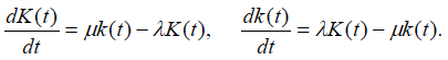
Availability index. In the theory of reliability of repairable items, one can consider failures and restorations (repairs) as a flow of events that starts at random moments of time and lasts for random durations of time. Let us assume that failures are rare events, that the process of failures and restorations is characterized by a constant failure rate λ (steady-state portion of the bathtub curve), that the probability of occurrence of n failures during the time t follows the Poisson’s distribution
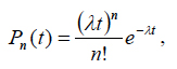 (1)
(1)
(see, e.g., Suhir1), that the restoration time t is an exponentially distributed random variable, so that its probability density distribution function is
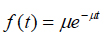 (2)
(2)
where the intensity

of the restoration process is reciprocal to the mean value of the process. The distribution (2) is particularly applicable when the restorations are carried out swiftly, and the number of restorations (repairs) reduces when their duration increases.
Let K(t) be the probability that the product is in the working condition, and k(t) is the probability that it is in the idle condition. When considering random processes with discrete states and continuous time, it is assumed that the transitions of the system S from the state si to the state sj are defined by transition probabilities λij. If the governing flow of events is of Poisson’s type, the random process is a Markovian process, and the probability of state pi(t) = P{S(t) = si,} i = 1,2...,n of such a process, i.e., the probability that the system S is in the state si at the moment of time t, can be found from the Kolmogorov’s equation (see, e.g., Suhir1)
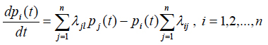 (3)
(3)
Applying this equation to the processes (1) and (2), one can obtain the following equations for the probabilities K(t) and k(t):
 (4)
(4)
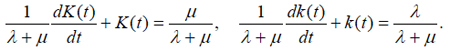
The probability normalization condition requires that the relationship K(t) + k(t) =1 takes place for any moment of time. Then the probabilities K(t) and k(t) in the equations (4) can be separated:
 (5)
(5)
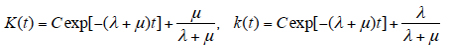
These equations have the following solutions:
 (6)
(6)
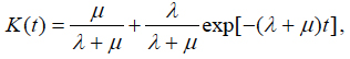
The constant C of integration is determined from the initial conditions, depending on whether the item is in the working or in the idle condition at the initial moment of time. If it is in the working condition, the initial conditions K(0) = 1 and k(0) = 0 should be used, and

If the item is in the idle condition, the initial conditions K(0) = 0 and k(0) = 1 should be used, and

Thus, the availability function can be expressed as
 (7)
(7)
if the item is in the working condition at the initial moment of time, and as
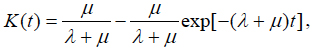 (8)
(8)
if the item is idle at the initial moment of time. The constant part
 (9)
(9)
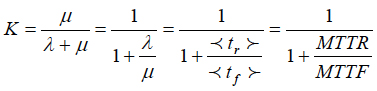
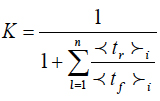
of the equations (7) and (8) is known as availability index. It determines the percentage of time, in which the item is in workable (available) condition. In the formula (9),
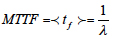
is the mean time to failure, and
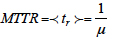
is the mean time to repair. If the system consists of many items, the formula (9) can be generalized as follows:
 (10)
(10)
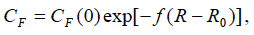
Minimized reliability cost. Let us assume that the cost of achieving and improving reliability can be estimated based on an exponential formula
 (11)
(11)
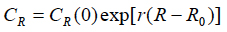
where R = MTTF is the reliability level, assessed, e.g., by the actual level of the MTTF; R0 is the specified MTTF value; CR(0) is the cost of achieving the R0 level of reliability, and r is the factor of the reliability improvement cost. Similarly, let us assume that the cost of reliability restoration (repair) also can be assessed by an exponential formula
 (12)
(12)
where CF(0) is the cost of restoring the product’s reliability, and f is the factor of the reliability restoration (repair) cost. The formula (12) reflects an assumption that the cost of repair is smaller for an item of higher reliability.
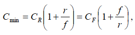
The total cost
 (13)
(13)
has its minimum
 (14)
(14)
when the minimization condition  is fulfilled. Let us further assume that the factor r of the reliability improvement cost is inversely proportional to the MTTF, and the factor f of the reliability restoration cost is inversely proportional to the MTTR. Then the formula (14) yields
 (16)
(16)
where the availability index K is expressed by the formula (9). This result establishes the relationship between the minimum total cost of achieving and maintaining (restoring) the adequate reliability level and the availability index. It quantifies the intuitively obvious fact that this cost depends on both the direct costs and the availability index. From (16) we have
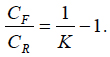 (17)
(17)
This formula indicates that if the availability index is high, the ratio of the cost of repairs to the cost aimed at improved reliability is low. When the availability index is low, this ratio is high. Again, this intuitively obvious result is quantified by the obtained simple relationship. The formula (16) can be used, particularly, to interpret the availability index from the cost-effectiveness point of view; the index reflects the ratio of the cost of improving reliability to the minimum total cost of the item associated with its reliability level.
The relationship between the availability index and cost-effectiveness of the product is quantified, assuming that the cost of improving reliability over its specified level increases, and the restoration (repair) cost decreases, when reliability level (assessed in our analysis by the mean-time-to-failure) increases. It has been shown that the total cost of improving and maintaining reliability can be minimized, and that such a minimized cost is inversely proportional to the availability index. The developed model can be of help when there is a need to minimize costs without compromising reliability.
References
1. E. Suhir, Applied Probability for Engineers and Scientists, McGraw-Hill, New York, 1997.
2. E. Suhir, R. Mahajan, A. Lucero and L. Bechou, “Probabilistic Design for Reliability (PDfR) and a Novel Approach to Qualification Testing (QT),” IEEE/AIAA Aerospace Conference, March 2012.
Ephraim Suhir, Ph.D., is Distinguished Member of Technical Staff (retired), Bell Laboratories’ Physical Sciences and Engineering Research Division, and is a professor with the University of California, Santa Cruz, University of Maryland, and ERS Co.; This email address is being protected from spambots. You need JavaScript enabled to view it.. Laurent Bechou, PH.D., is a professor at the University of Bordeaux IMS Laboratory, Reliability Group.