The first men to investigate the maximum current a copper conductor can carry before it starts to melt devised lasting equations.
As circuits continue to get more powerful and also denser, the power handling capability of some of our PCB traces becomes more important. IPC-2152, Standard for Determining Current Carrying Capacity in Printed Board Design,1 was a major step forward in helping board designers deal with these issues. But sometimes there is a power handling issue that falls outside the scope of IPC-2152.
For example, consider the situation where a trace normally carries a modest current (and therefore can be a modest size). If there is a catastrophic system failure that trace may be subjected to a major current overload. It is important that the trace maintain its integrity for a short period of time (say, one or two seconds) while the system goes through an automatic, controlled system shutdown. The trace need only to carry that current overload that short time without melting. So the question becomes, how big a trace do we need?
The maximum current a conductor can carry before it starts to melt is called the “fusing current.” The first people typically credited with looking into this question for copper conductors are William H. Preece and I. M. Onderdonk. This article looks at who Preece and Onderdonk were, what (apparently) motivated them, and where basic source materials can be located. Finally, in the absence of a source document by Onderdonk himself, we offer a derivation of his well-known equation.
W H. Preece
During the 1880s, Sir William Henry Preece was a consulting engineer for the British General Post Office. At that time, the Post Office was responsible for the telegraph (and later wireless telegraph) system in England. He published three papers in the Proceedings of the Royal Society of London in the 1880s that formed the basis for his famous equation
I = a * d3/2 [Eq. 1]
where d is the diameter of the wire in inches; a is a constant (10244 for copper), and I is the fusing current in amps. A little algebra transforms this equation to
I = 12277*A3/4 [Eq. 2]
where A is the cross-sectional area in inches2.
Until recently it was very difficult to get copies of these three papers. In recent years, the Royal Society of London has made its archives available online.2 The first of the papers, 1883, poses the problem Preece was interested in. The coefficient for copper (10244) is found in his third paper (1888).
I. M. Onderdonk
To the best of our knowledge, no original source document for Onderdonk’s Equation exists. Who I. M. Onderdonk was remains a mystery. The earliest reference to him we are aware of is in a 1928 article by E. R. Stauffacher in the General Electric Review.3 At that time, Stauffacher was superintendent of protection at Southern California Edison. That article references Onderdonk’s Equation as
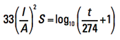 [Eq. 3]
for a reference temperature of T = 40°C. Some later publications offer a more general form:
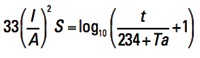 [Eq. 3a]
where:
I = current in amps
A = cross-sectional area in circular mils (Note 1)
S = time in seconds the current is applied
t = rise in temperature from the ambient or initial state (see Note 2)
Ta = reference temperature in ˚C
If we compare the results of Onderdonk’s and Preece’s equations for any conductor, we get somewhat similar outcomes. But Onderdonk’s Equation has the additional benefit that there is a variable “time” included. Thus we can calculate a “fusing current” for any conductor based on the time the conductor must carry the current, within reasonable limits. (See below.)
Motivations. Preece’s and Onderdonk’s motivations were similar. Preece’s motivation is clear from his 1883 paper. He was concerned about the effects a lightning strike might have on the telegraphy equipment. They did have, back then, an early form of a lightning arrestor. As part of it there was a wire link that acted as a fuse. Preece wanted to know the best material and size for this wire link, so that the fuse would carry the normal amount of current for telegraphic operation, but would melt under the effects of a lightning strike. Although, as a result of his experiments, he concluded that “the best metal to use for small diameters was platinum, and for large wires tin” (1887); his final constants for all materials, including copper, are found in his 1888 paper.
Since Stauffacher’s article is the first reference we know of regarding Onderdonk, it is tempting to speculate that he was an associate of Onderdonk. Perhaps Onderdonk was also an employee at SCE. Stauffacher’s article describes the problem of a short-circuit current across an insulator in a high-voltage transmission line. A nomograph in that article credited to Onderdonk has values consistent with this type of problem. The copper wires supporting the insulators and the poles had to be able to carry this short-circuit current for enough time for the automatic switching equipment to isolate the power line.
Both problems require a conductor to carry a high-voltage, high-current spike for a short period of time.
Derivation. Because no original source seems to exist for Onderdonk’s Equation, the authors offer the following derivation (see Note 3):
Step 1. The joule heating of a conductor by electrical current is R *I2* Δt, where R is resistance in ohms; I is current in amps, and Δt is the time in seconds the trace is heated. We are explicitly assuming there is no cooling of the trace due to conduction, convection or radiation, so Δt is necessarily short.
Now we know that resistance is given by ρ*L/A, where ρ is the resistivity of the conductor material; A is the cross-sectional area of the conductor (in square m), and L is the length of the conductor (also in m.) But ρ is a function of temperature. When we adjust for changing temperature, the formula for resistance is
R = ρA * (1 + αA * (T-TA))*L/A [Eq. 4]
where:
ρA is the resistivity at any reference temperature
αA is the temperature coefficient of resistivity at the reference temperature
T-TA is the change in temperature from the reference temperature, TA.
Putting all this together, the joule heating of a conductor by electrical current is
ρA * (1 + αA * (T-TA)) * (L/A) * I2 * Δt [Eq. 5]
Step 2. The gain of thermal energy of the same conductor is cp * M * (T – TA) where cp is the specific heat capacity of copper, and M is the mass of the conductor. Furthermore, mass can be expressed as ρ * A * L, where this ρ is the density of copper (not to be confused with resistivity). Putting all that together results in the gain of thermal energy as
cp * ρ * A * L * (T – TA) [Eq. 6]
Step 3. The units of Eq. 5 and 6 are the same (joule = W*sec). Therefore, Eq. 5 and Eq. 6 are equal to each other. If we let (T – TA) = Τ and let the Ls cancel, we can write
cp * ρ * A * Τ = ρA * (1 + αA * Τ) * (I2/A) * Δt [Eq. 7]
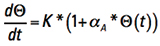
Now, recognize that Τ is inherently a function of time, or is time dependent. We can let Δt become the calculus dt, rearrange terms, and form the ordinary differential equation
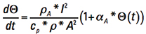 [Eq. 8]
We can simplify the way this looks by temporarily recognizing the first term on the right is a constant with respect to t and let 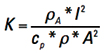 .
.
Then we can express Eq. 8 in more friendly terms
 [Eq. 9]
Remember when teachers used to say, “It is left for the student to show?” Well, the steps to the solution to this differential equation are beyond the scope of this article (see again Note 3). But the solution is (assuming time starts at t = 0 and Τ =0)
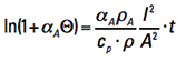 [Eq. 10]
Step 4. Changing sides and moving αA to the denominator, for reasons that will be apparent in a moment, we get
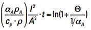 [Eq. 11]
Now let us look at the term inside the parentheses on the left side. They are all constants. To evaluate them, recognize first that the product of α * ρ is a constant for any temperature (see again Note 3). So
αA * ρA = α20 * ρ20 [Eq. 12]
Plugging in the appropriate constants, we get Eq. 13
α20 = 0.00393 1/K
ρ20 = 1.75×10⁻⁸ Σ m²/m
cp = 385 J/kgK
ρ = 8900 kg/m³
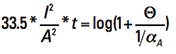
 [Eq. 13]
This equation is in metric units and natural logarithm. To convert it to circular mils (because that is the form of Onderdonk’s Equation) and Log10, recognize the following relationships:
1 m² =1.98 109 circ-mils
to go from ln to log10 we have to divide by ln (10) = 2.30
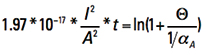
This results in
 [Eq. 14]
Finally, from Eq. 12 we can look at 1/αA and derive that
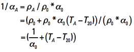
This last line evaluates to 1/αA = (1/0.00393) + TA – 20 = 234 + TA . So, finally, Eq. 14 becomes
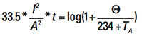 [Eq. 15]
Eq. 15 is almost exactly Onderdonk’s Equation as shown in Eq. 3a.
Other units. If we rearrange the terms of Eq. 15 and recognize the melting temperature of copper is 1083˚C, we can obtain (in circular mils):
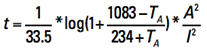 [Eq. 16]
If we further let the ambient temperature equal 20˚C, we can obtain:
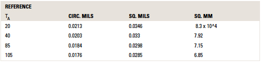
t = c * (A/I)2 [Eq. 17]
where c = 0.0213 in circular mils.
The values for c in other units and at other reference temperatures are provided in TABLE 1.
Table 1. Values for C for Areas in Various Units
Cautions. There are two time periods to discuss when talking about “fusing” current. One is the time to reach the melting temperature of the material. A second is the time to actually melt the material after the melting temperature is reached. The literature is somewhat careless about how it refers to the “melting” time or “fusing” time of a material. But it is clear from reading Preece’s article and from the Onderdonk derivation that both Preece and Onderdonk are referring to the first time, the time to just reach the melting temperature of the material.
When we started with Eq. 5 we had explicitly assumed there was no cooling of the conductor. In the real world there will be some cooling fairly quickly. If some cooling is allowed for, that means it will take longer for the trace to reach the fusing temperature. Thus, Onderdonk’s Equation is valid only for a short period of time. The references quoting Onderdonk’s Equation typically say it is no longer valid after 10 sec. Adam5 argues that the time is much shorter, probably no longer than one to two sec.
Notes
1. A circular mil is the area of a circle with a diameter of one mil. The formula is A = d2. The conversion from circular mils to mil2 is π/4. Normal conversions are:
1 mil2 = 1.273 circular mils
1 circular mil = 0.7854 mil2
1 m2 = 19.736*108 circular mil
1 circular mil = 5.067*10-10 m2 = 5.067*10^-4 mm2
2. From a thermodynamic engineering standpoint there is a significant difference between ambient temperature and initial condition. For example, there could be some heating of a conductor above the ambient temperature in a normal operation before a change of current is applied. In this paper we assume the initial condition (temperature) is the same as the ambient temperature.
3. Parts of this derivation are summarized. For a complete derivation, including all steps, see Adam and Brooks4 and Adam5. Since Dr. Adam (from Germany) provided the initial work on this derivation, the constants are in metric units. We convert them to their imperial equivalents at the end of the derivation.
References
1. IPC-2152, Standard for Determining Current Carrying Capacity in Printed Board Design, August 2009.
2. W. H. Preece, “On the Heating Effects of Electric Currents,” Proc. Royal Society 36, 464-471 (1883). No. II, 43, 280-295 (1887). No. III, 44, 109-111 (1888).These documents have been made available online in recent years:
http://rspl.royalsocietypublishing.org/content/36/228-231/464.full.pdf+html
http://rspl.royalsocietypublishing.org/content/43/258-265/280.full.pdf+html
http://rspl.royalsocietypublishing.org/content/44/266-272/109.full.pdf+html
or at www.ultracad.com/articles/reprints/preece.zip
3 E. R. Stauffacher, “Short-time Current Carrying Capacity of Copper Wire,” General Electric Review, vol. 31, no. 6, June 1928 (ultracad.com/articles/reprints/stauffacher.pdf).
4. Johannes Adam, Ph.D. and Douglas Brooks, Ph.D., “In Search of Preece and Onderdonk,” available in the “Articles” section at www.ultracad.com/articles/preece.pdf.
5. Johannes Adam, Ph.D., “The Adiabatic Wire: ‘Onderdonk,’ ” white paper No.10 at www.adam-research.de/pdfs/TRM_WhitePaper10_AdiabaticWire.pdf.
Douglas Brooks, Ph.D., is owner of UltraCAD Design, a PCB design service bureau and author of PCB Currents: How They Flow, How They React; This email address is being protected from spambots. You need JavaScript enabled to view it.. He will speak at PCB West in September in Santa Clara, CA. Johannes Adam, Ph.D., CID, is founder of ADAM Research, a technical consultant for electronics companies and a software developer, and the author of the Thermal Risk Management simulation program.
Ed. note: Due to a conversion error in the editorial layout process, the rho symbol (ρ) was inadvertently converted to a pi (π) symbol in the print version of this article. The editors regret the error.