How to calculate PCB trace width and differential pair separation, based on the impedance requirement and other parameters.
Impedance control is about accuracy. If one or two parameters are not carefully determined, we can lose the advantage of the more accurate parts of the process (for example, the usage of the expensive field solver programs). With simulators and calculators, we can determine trace width impedance (used for analysis) or impedance trace width (used for design). The calculations also depend on other parameters, but the role of width and impedance determines the usage. To get the best accuracy, perform full frequency-dependent impedance control. Even if we use the simplier and less expensive frequency independent design flow, it is worth it to understand the simplifications we make.
The proposed design flow: Calculate PCB trace width and differential pair separation based on the impedance requirement and other parameters (FIGURE 1).

Input parameters needed:
- Impedance requirement
- Materials and thicknesses (PCB fab stock)
- Dielectric Dk and Df on a given frequency
- Soldermask data, Dk and Df on a given frequency
- Etching compensation data from PCB fab
- Signal knee frequency
- Copper and plating thicknesses.
We need a frequency-dependent 2D field solver program, like the Polar Instruments Si9000 or Appcad RLGC. A frequency-independent (less expensive) field-solver, like the Plar Si8000 or TNT-MMTL, can get 1% to 5% error.
The field solver program itself is not enough. We also need to do additional calculations such as Dk and Df on the signal’s knee frequency (this can be done in an Excel calculator) and the CAD_width and CAD_separation from the field-solver results.
All parameters have tolerances, including the calculation itself, the manufacturing and the measurements. To achieve a reasonable accuracy, we need to minimize all the tolerances so that in total, they fall within specified limits (usually 10% or 15%). Even if a few parameters have loose tolerances, keep tight tolerances where possible. For example, for a worst-case calculation: Parameter A has 1% (simplified case, truncated distribution) tolerance, Parameter B has 1% to 10% (10% is with less expensive equipment) tolerance, Parameter C is fixed at 10%. If we choose 10% for Parameter B, then the total worst case tolerance will be 21%. If we choose 1%, then the total will be only 12%, which is much lower. If we specify our nominal impedance with a loose tolerance (choosing 90-ohms nominal for a 100-ohms diffpair) manufactured at +/-10%, together they will result in a 90 ohms +/-10% (81 to 99 ohms) range, which is outside of our original specification (100+/-10% = 90 to 110 ohms).
The PCB manufacturer measures the test coupons on each panel, not each trace on each board. The dielectric and copper thicknesses are not perfectly equal everywhere on the panel, so the real traces will also have a deviation from the test coupon measurement results. This can be minimized by providing similar copper pattern and density on the coupons as the board design.
It is common for manufacturers to have an error in one parameter (for example, under etching) during calculations, so they can modify another unrelated parameter (for example, the Dk) to push the calculation results close to the measured values. If we try to correct the modified parameter, we will get a result different from the measurements, which means our calculations will be incorrect.
Dielectric materials. Materials have a part number (for example, Isola IS410), but that number does not specify the material for an impedance calculation. An exact material specification example would be: Isola IS410, 2116 glass style, 125-um finished thickness prepreg, 67% resin content. The materials are available in a few specific thicknesses, with each thickness variant having a different dielectric constant and loss tangent; therefore, we need to know the exact Dk and Df. A common mistake is to use the Dk and Df data from the material datasheet, which can have up to 20% difference to the value of the chosen thickness variant. It is worth buliding a material library, since it is hard to get those material Dk and Df values for each thickness. Normally, these are measured or calculated based on the resin content.
Dk is a function of frequency, and the material manufacturers specify the Dk and Df data on a certain fixed frequency (usually on 1 MHz, 1 GHz or 5 GHz). Both strongly change over the frequency, so derive their values on the signal’s knee frequency. The slope of the Dk curve depends on the Df value, a higher Df leads to a bigger change in Dk over frequency. The compensation can be done with analitical equations (in an Excel sheet) based on the wide band Debye model.
Etching compensation. The etching compensation has to be done at two points in the calculation. For both, we need some values from the PCB manufacturer, since it is a manufacturer-dependent value.
With some simplification, the PCB signal trace cross-section can be modeled as a trapezoid. Before ething, the manufacturer creates an acid-resistant pattern on the copper surface, where the track widths are exactly the same as in the PCB artwork files. Let’s refer to the trace width in the design files as CAD_width. During etching, the final trace will be narrower than the CAD_width, and the topside width (Top_width) will be narrower than the bottomside (Bottom_width). This has the opposite effect on the trace separation, which is important for differential pairs. Which one is the top/bottom? During etching, the copper foil is already applied to the surface of one of the dielectric layers. The other dielectric layer will be added after the etching. So, the side of the trapezoid touching the existing dielectric layer (core or earlier prepreg) will be the wider one, and it will be the usually called Bottom_width (FIGURE 2).

We need to get two values from the manufacturer for a given copper thickness:
We need the difference between the Top_width and the Bottom_width, referred to as “lower trace width etch factor” in Polar Instruments’ terminology. We will call it Etch_Factor_1 and provide this to the field-solver program.5
We need the difference between the Bottom_width and the CAD_width; let’s call it Etch_Factor_2.
These are statistical-measured average values. If the manufacturer doesn’t provide these numbers, then we can assume that:
Etch_Factor_1 = Etch_Factor_2 = copper_thickness 0.6, so it is dependent on the copper thickness.
Polar Instruments Si8000 software deals only with Etch_Factor_1, so we have to calculate the final CAD_width and CAD_separation manually:
CAD_width = Bottom_width + Etch_Factor_2
CAD_separation = Bottom_separation - Etch_Factor_2
Some manufacturers calculate the final CAD_width, some don’t. For this reason, before setting up trace widths in the CAD design program, ask the fab house if it does this final compensation. If it does, set up the Bottom_width for the CAD program; if it doesn’t, then set up the CAD_width (or photomask width) for the layout.
Buildup order. The copper layer is always between two dielectric layers (inner) or ontop of a dielectric layer (outer). For the inner layers, before etching, the copper foil is already on the surface of one of the dielectrics, which is hard already (core, or earlier prepreg in a buildup-type microvia stackup). After the circuit is etched the next prepreg (dialectric) layer is applied and cured. The result is that the copper pattern is embedded into the second (soft, prepreg) layer. The wider part of the trace cross-section is on the surface of the hard layer. The upper and lower dielectric in the structure view is not based on the board orientation or layer number, but on the core prepreg or buildup order (FIGURE 3).

Copper coverage. The ratio of the remaining copper to the removed copper on a given layer is the copper coverage. It has an effect on the final thickness of the prepregs. If there is less copper remaining, less copper will be embedded into the prepreg and less volume will be added to the prepreg’s volume. The prepreg flows slightly during the lamination process and fills the gaps between the traces horizontally. The board surface area is constant, so if one layer’s volume increases then its thickness also increases.
Naming conventions. The finished thickness is the thickness of a prepreg layer when it is laminated between 100% fully covered copper layers. So in case of no copper embedding, it can be used for the prepreg volume calculation. Because this name is already occupied, name the resulting prepreg thickness in the stackup as “final thickness.” Note that we measure the prepreg final thickness not from the top of the traces, but from hard/full layer surface (core, or earlier prepreg, or ground/power plane) to another hard/full layer. The Polar software uses the “isolation distance” naming for this.6
Finished prepreg thickness for buildups:
Final_thickness = finished_thickness + coverage * copper_thickness
For core-prepreg sandwiches:
Final_thickness = finished_thickness + coverage1 * copper_thickness1 + coverage2 * copper_thickness2
Both sides of the prepreg have embedding copper patterns. FIGURE 4 illustrates copper patterns for different stickups.

Plating. For outer copper layers where any drilled holes are ending, the manufacturer increases the copper thickness with copper and other metal plating to create the plated through-holes (PTH) and to make the outer surfaces easily solderable. This increases the layers’ thickness and must be taken into account for impedance calculations. These thickness measurement data can be requested from the manufacturer. If we change manufacturers in the product’s lifetime, then the plating thicknesses also change, so all impedances must be recalculated. For some PCB manufacturing processes, the plating also results in a more complex shaped cross-section, resembling a mushroom rather than a trapezoid.
Frequency dependence of the characteristic impedance. The characteristic impedance is defined in the well-known equation:

The “j” is the complex-number constant, f is the frequency and the R, L, G and C parameters are per-unit-length parameters (each also frequency dependent) derived by solving the electromagnetics differential equations (this is what a field-solver does). The result Z0 is a complex number on every frequency. We take the magnitude of this complex number, so that is why we say “impedance magnitude.”
The trace impedance depends on the frequency, because of the following effects: Dk is frequency dependent (effects C, G), skin-effect (effects L, R).
At very low frequencies, around 30 MHz, the impedance rapidly increases with decreasing frequency. Above that region, the slope can be positive or negative, based on the cumulative result of all of the parameters. In most of the digital circuits, we don’t care about the impedance at that level (below 30 MHz) frequencies. Above 10 GHz to 100 GHz, it increases rapidly again. FIGURE 5 illustrates impedance magnitude vs. frequency for a 100-μm wide microstrip on an 100 μm-thick dielectric.

Frequency dependence of the digital signals. Digital signals are wide-band signals. However, the rest of the signal’s energy is located in a not too wide frequency band. For 8b10b encoded signals, like the PCI-express and SATA, the frequency band has a lower limit, which is one-tenth of the data rate (FIGURE 6). The highest significant frequency component of a digital signal is at the knee frequency. F_knee = 0.5 / Rise_time. To minimize signal integrity problems, it would make sense to provide the best matched termination at the knee frequency.

The rise time is normally slower (lower knee frequency) at the receiver circuit than at the transmitter, due to losses and attenuation in the interconnect. If we have to choose where to have better match, at the transmitter or at the receiver, then we have to answer this question before we start the impedance calculation. Because of the different rise times, the two ends of the signal trace will see different impedance as well. Ideal termination is obtained when the terminating resistors resistance is equal (neglecting the complex nature of the impedances) to the local characteristic impedance.
Surface roughness. The surfaces of the copper and dielectric layers are not perfectly flat and smooth. They have a roughness usually a few micrometers deep. For signal frequencies where the skin depth (skin effect) is at least as low as the surface roughness, it increases the effective trace length and the series resistance of the trace [R(f)], too (FIGURE 7). This way, it has an effect on characteristic impedance.6

Soldermask. The soldermask must be taken into account for outer layer microstrip calculations. It has a Dk and Df similar to the other dielectrics in the stackup. These parameters can be obtained from the soldermask datasheet.
Soldermask thickness. We deal with multiple soldermask thicknesses and provide the thickness ontop of the copper traces and the thickness between the traces. We can also provide the conformal coating thicknesses, if they exist.
Other effects. There are several other aspects of the characteristic impedances what we could analyze, but there is no developed method to take them into account in our calculations in the design process.
Fiber wave effect. The PCB dielectric materials are not homogenous; they are a mix of glass fibers and resin not perfectly distributed. These two components have very different dielectric constants. If a PCB trace is parallel to a glass fiber direction, the location of the trace relative to the glass fiber determines the effective Dk around the trace, and the impedance will depend on the relative location. The imperfect glass-resin distribution pattern provides the same dielectric constant offset (and impedance offset) through the whole length of the trace, which is the worst case. However, if the traces are in some angle to the glass thread direction, then the error appears as a fluctuation over the length with a mean value of the nominal dielectric constant, which is the desired way. FR-4 materials have glass fiber threads in two directions, just like the yarns in a fabric. To be able to have the traces in angle to both thread directions, route the traces to be 45˚ to both fiber directions.8
Geometry roughness. The trace width, dielectric thickness and all edges and surfaces in the geometry are neither perfect nor smooth. On a longer trace, we can observe the mean value of these otherwise statistically natured geometry parameters/dimensions.
Resin flow. Since the PCB dielectrics are made of glass fiber and resin, the resin flows slightly and fills gaps between traces after the lamination process.This way between the traces on the same layer there will be almost only resin. There will be areas filled more with resin and other areas filled more with glass, this way the dielectric constant will vary from area to area. The FR4 dielectric constant is a result of the dielectric constants of the glass fibers and the resin, but in areas where it is no longer a mix but just resin, the dielectric constalt is a lot different than the nominal value as provided for the material.9
References
2. “Frequency Domain Characterisation of Power Distribution Networks”, Istvan Novak, Jason R. Miller, p.106.
3. “Modeling frequency-dependent dielectric loss and dispersion for multi-gigabit data channels,” Simbeor Application Note #2008_06, September 2008.
4. The following is an Excel sheet for recalculating the Dk data to different frequencies: www.buenos.extra.hu/iromanyok/E_r_frequency_compensation.xls. It is based on equations from Istvan Novak’s demonstrating caclulator: “causal frequency dependent dielectric constant and loss tangent dielectric model parameters,” http://electrical-integrity.com.
5. Polar Instruments, www.polarinstruments.com.
6. AP507, “Calculating dielectric height with Speedstack,” www.polarinstruments.com/support/stackup/AP507.html.
7. “Surface roughness effect on PCB trace attenuation / loss,” Polar Instruments Application Note AP8155.
8. Altera application note 528: “PCB Dielectric Material Selection and Fiber Weave Effect on High-Speed Channel Routing,” www.altera.com/literature/an/an528.pdf.
9. AP148, “The Effect of Etch Taper, Prepreg and Resin Flow on the Value of the Differential Impedance,” www.polarinstruments.com/support/cits/AP148.pdf.
Istvan Nagy is a hardware design engineer with Concurrent Technologies; This email address is being protected from spambots. You need JavaScript enabled to view it..