By following three key guidelines, it is possible to achieve a better that two-percent agreement between measured and simulated high-speed performance.

There is a methodology for evaluating the accuracy of field solver tools that translate the geometry and material properties of uniform interconnects into their high speed S-Parameter behavior.¹ An accurate simulator can be an invaluable tool to efficiently explore design space for the best cost-performance trade off, but evaluating the accuracy of the simulation tool is tricky. When “as designed” geometry and material properties are used as input to the Polar Instruments Si9000 transmission line simulator, no better than a 10% agreement can be expected. However, when accurate input information is used, the accuracy of the Si9000 S-parameter predictions is better than 2%.

The Power of Simulation

Practical product design is about balancing three different requirements: acceptable performance; a tight schedule; and cost efficiency. It’s easy meeting any two of these requirements, but it’s a challenge meeting all three at the same time.

With our globally competitive design environment, if your design team isn’t able to get the lowest cost product to market in the shortest time, your competition will.

A common practice in meeting difficult performance targets is to “buy insurance” by paying extra for added design margin. The greater your uncertainty in the actual performance of your product and the lower your risk tolerance, the more margin you are inclined to buy. This can appear as more board layers, lower loss laminate materials, a tighter tolerance for line impedance, more decoupling capacitors or more expensive transceivers.

Sometimes, these more expensive features are worth the extra cost in gaining you the performance edge in “extreme tech” products. But, most of the time, the question is how do you achieve “acceptable” performance targets with products designed right the first time, that have a minimum of extra margin?

This is where an accurate simulation tool can increase your confidence and allow you to have the same low risk without buying more design margin than you need to compensate for component and manufacturing variations.

There is no substitute for creativity and imagination in the initial design phases of any project, but, an accurate, versatile simulator tool can be a virtual prototyping station, allowing you to spin through multiple design cycles to find the optimum cost-performance trade off faster and cheaper than spinning hardware designs. A key condition of the simulation tool, however, is accuracy.

Evaluating the Accuracy of Transmission Line Simulation Tools

There are four approaches to gaining confidence in the accuracy of an analysis tool:

• Compare the results to analytically exact equations.
• Compare the results to other, well- established industry standard simulation tools.
• Compare the results to well characterized test vehicles.
• Compare the results to typical interconnect structures.

This last step is usually what is done to gain confidence in the accuracy of a tool because it is easy. However, when you take a circuit board trace on a board, try to simulate its performance and then compare the simulated results to a set of measured results, the difference between the two is often not a measure of the accuracy of the tool but of the accuracy of the values of the material properties and the fabricated geometrical features.

Such a comparison is more a measure of the practical ability to design and to fabricate for a targeted performance parameter than the accuracy of the simulation tool. This is important information, but often times, the direction to follow in order to get closer to the target value is not “improving” the accuracy of the simulation tool but controlling the fabrication processes. This gives rise to variations between the “as designed” values and the “as manufactured” values, as well as inaccuracies in the values of the material properties.

While the characteristic impedance or differential impedance are important design goals and are straightforward to measure, a more general metric of transmission line performance is the S-Parameter matrix from each port or end. These elements will typically span a frequency range from 10 MHz to above 10 GHz. The S-Parameter values over this frequency range are strongly influenced not only by the impedance of the lines, but also by the coupling between adjacent lines and the losses in the lines.

Results From a Test Vehicle

A simple four-layer board was constructed with a variety of coupled lines. An example of a closely spaced stripline pair is shown in FIGURE 1.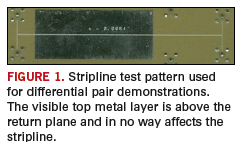



Of course, since these traces are buried between reference layers, they can’t be seen from the surface. A silkscreen pattern was used to illustrate the location of the buried traces. SMA launches from the back of the board, on 0.5 inch centers, connected to the VNA.

After a short length of uncoupled stripline trace, the traces come together into a tightly coupled region for a four-inch run. The nominal conditions, as designed, are shown in FIGURE 2. The dissipation factor was reported as 0.02. We asked the fab vendor, “What is the dissipation factor?” The fab vendor replied, “What do you expect?” We stated, “0.02.” The fab vendor replied, “Yes, that’s the value.”



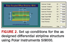
Obviously, the precise values of the geometry features and material properties will strongly influence the simulated performance of the interconnect. There are really three different sets of geometry and material property values: as design; from the fabricator; and as measured in reality.

Unfortunately, each of these will probably be different. The only way to do a measurement and an accurate comparison of a simulation tool is by using values for the geometry features and material properties from direct measurements of cross sections of the sample and specially designed test vehicles. This will extract the material properties.

The as designed nominal values were used as a starting place, with the material properties as reported by the fab vendor. A touchstone file was created using Polar Instruments Si9000 to represent the tightly coupled region.

This touchstone file was imported into Agilent’s Advanced Design Systems (ADS), a signal integrity and RF design tool, and compared with the S-Parameters in both the frequency domain and the time domain. The initial comparison is shown in FIGURE 3 for the case of the single-ended return and insertion loss of one line in the pair.



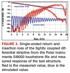
Clearly, there is a big difference, especially in the return loss, which is most sensitive to the impedance profile. A common reaction is that there must be something wrong with the simulator. Unfortunately, the real world is often far subtler than we would like it to be.

When we perform a measurement, we rarely measure exactly what we are simulating, unless we work very hard to match the conditions. In this example, what we are measuring is not only the uniform coupled stripline pair, but also the SMA launches and the uniform, uncoupled stripline feed section – but the touchstone file only has the long, uniform coupled stripline section.

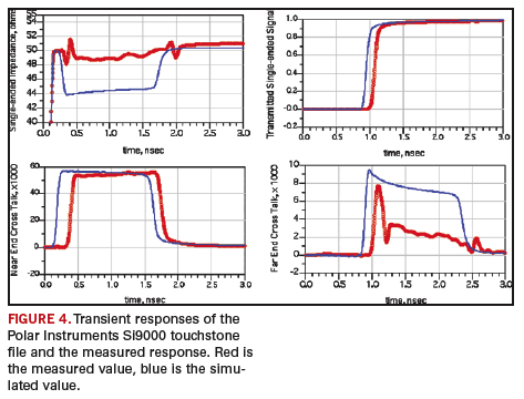
This difference between measured and modeled performance can clearly be seen by comparing the time domain measurement and simulation. The transient responses of the measured S-Parameters for the first column of elements and the simulated touchstone file from Polar Instruments Si9000 are shown in FIGURE 4. The transient responses show three important features lacking in the simulated response: discontinuities associated with the SMA launches, the extra uncoupled length of the connection from the SMA to the coupled stripline section and a large difference in the single-ended impedance between the measured and simulated values. In order to match the simulation condition to the measurement condition, an accurate model for these features must be included in the simulation.



It is possible to de-embed the launches using techniques such as TRL and circuit topology-based modeling. In general, the SMA launches can be modeled with short sections of uniform transmission lines. The uncoupled launch sections can be modeled as sections of uncoupled transmission line.²

When these elements are included in the model, but the same touchstone model with as designed parameters is used, the agreement, shown in FIGURE 5, is better but still not perfect. At this point, it is natural to think that this level of agreement is a measure of the accuracy of the simulator. After all, it is pretty close. The measured impedance seen in the TDR response is roughly 49 ohms, and the predicted impedance is 44 ohms, which is within 10%.



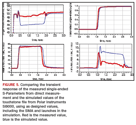
The general features of the near- and far-end cross talk are represented in the simulated response. However, the simulated touchstone file is based on using values for the geometry and materials, based on the as designed values.

Cross section measurements and a test structure designed to extract the dielectric properties indicted that the dielectric thickness of each layer was not 10 mils but 10.2 mils. The line width was not 8.6 mils but was etched back to 8.0 mils. This increased the spacing from 8.4 mils to 9 mils. The pitch, of course, was not affected by the etch back. The dielectric constant was measured as 4.0 from a test structure, not 4.5 as reported by the fabricator. However, the dissipation factor was measured to be 0.02.

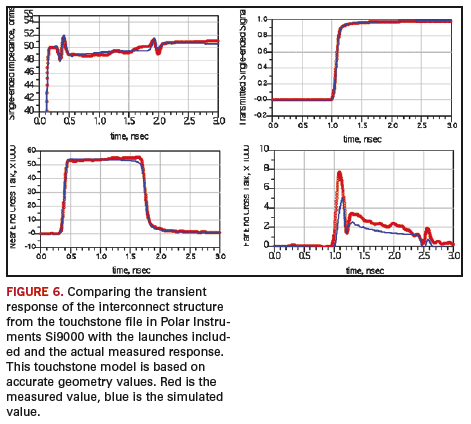
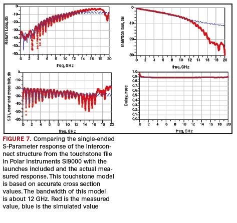
A new touchstone file from Polar Instruments Si9000 was generated based on these as measured values and re-simulated to compare with the measured S-Parameters, including the model of the SMA and short transmission line launches. The final comparison is shown in FIGURES 6 and 7.
This exercise illustrates that, with careful analysis, excellent agreement can be achieved between the measured performance of real physical systems and the predicted performance from the Polar Instruments Si9000 simulation tool–up to at least 12 GHz.

Conclusion

In order to accurately predict the measured performance of real structures, three important guidelines should be followed:

Simulate exactly the same configuration as is being measured, including the launches, vias, feed lines and other features. Alternatively, de-embed all connectors, launches and feeds so that the measurement is exactly the same as the structure being simulated.

If the interconnect being measured has any discontinuities or losses, do not read the impedance values directly off the front screen of the time domain reflected response as the accurate lossless impedance. These features complicate the interpretation of the displayed values.

For accurate correlation, use geometry values from cross section measurements and material properties from direct measurements of test vehicles.

If these guidelines are not followed, then at best, one might expect 10% agreement between measured and simulated performance, but this is more a measure of the accuracy of the geometry and material values. If care is taken and these guidelines are followed, it is routinely possible to achieve better than 2% agreement between a predicted response and a measured response well above 10 GHz. PCD&F

References

Signal and Power Integrity – Simplified, Eric Bogatin, published by Prentice Hall, 2009.
OnLine Lecture OLL-691 “Building High Bandwidth Models from Measurements,” www.beTheSignal.com

Dr. Eric Bogatin is president of Bogatin Enterprises, LLC.  He can be reached at This email address is being protected from spambots. You need JavaScript enabled to view it..